{
    "version": "https://jsonfeed.org/version/1",
    "title": "Murto Hilali - Compbio, tech, proteins, and more.",
    "home_page_url": "https://murto.co/",
    "feed_url": "https://murto.co/feed.json",
    "description": "My digital garden & portfolio. I write about computational biology, tech, proteins, and more.",
    "icon": "https://murto.co/favicon.png",
    "favicon": "https://murto.co/favicon.ico",
    "expired": false,
    
    "author":  {
        "name": "Murto Hilali",
        "url": "https://murto.co/",
        "avatar": "https://murto.co/img/author/website-headshot.jpeg"
    },
    
"items": [
    
        {
            "id": "https://murto.co/acarbose-alternative-drug-discovery/",
            "title": "How I Found 71 Natural Alternatives to a $200 Million Drug",
            "summary": "A step-by-step drug discovery and AI virtual screening project done from my laptop",
            "content_text": "By Author — Not random images either, there’s a chance you find the compounds in all of these organisms.Table of Contents  Exploratory Data Analysis for COCONUT — Profiling ~100K natural products to understand drug-likeness, physicochemical space, and screening viability.  Chemical Similarity Search — Fingerprint-based filtering (ECFP, MACCS, pharmacophore, USRCAT) to reduce the database to high-similarity candidates.  Protein Model Selection, Cleanup, and Preprocessing — Selecting acarbose-bound crystal structures and preparing them for docking.  Protein–Ligand Docking &amp; Assessment — Running GNINA-based virtual screening and scoring with CNN-VS.  Lead Validation and Controls — Decoys, redocking replicates, statistical filtering, and stability analysis to remove false positives.  Candidate Overview &amp; Key Takeaways — Final shortlist by target protein and reflections on the workflow.Flavonoids are a large, diverse group of secondary plant metabolites that play a role in pigmentation, UV protection, and insecticidal activity. Specifically, some anthocyanins (a subclass) can inhibit insect digestive enzymes, preventing nutrient uptake and development, serving as a defence mechanism against predators.Obviously, there’s potential here for bug Ozempic (or insecticides, you pick). But research on Allium mongolicum flowers has also revealed that their flavonoids may inhibit human digestive enzymes, including our very own starch-metabolizing α-glucosidase. These compounds could be used to treat diabetes, as inhibiting starch breakdown reduces postprandial blood glucose levels (Li et al., 2025).Initial docking analysis revealed that A. mongolicum-derived isoquercetin (already in clinical trials) can inhibit α-glucosidase (AGI) activity with an effect similar to that of acarbose , a common AGI derived from Actinoplanes bacteria. Chemical similarity search revealed that troxerutin (aka vitamin P4, a flavonoid you can buy over the counter) shares some substructural motifs with isoquercetin, and its docking analysis showed similar binding affinity.Docking results from DiffDock-Pocket.  Note : troxerutin’s slightly higher affinity may be attributed to steric interactions introduced by the moieties found on the larger molecule.I wanted to take this approach and extend it to a larger database of natural compounds to find other biochemicals that could hypothetically outperform acarbose — after all, the drug is projected to have a $220 million global market by 2035.Here’s my overall process:      Exploratory data analysis of COCONUT, a natural products database.        Chemical similarity search of acarbose against COCONUT to find structurally similar NPs.        Protein model selection, cleanup, and preprocessing.        Protein-ligand docking and assessment , where I run a virtual screen against human α-glucosidases.        Lead validation and controls to identify any false positives.  You can see all the code (in progress) here. Workflow diagram1. Exploratory data analysis for COCONUTIn this section, I’ll take a look at:      Distributions of some pre-existing features in the database.        The spread of some derived ratios.  There are a little over 100,000 natural products in the COCONUT database. I started by doing some simple feature visualization:      Total atom count : all atoms, including hydrogen.        Heavy atom count : any non-hydrogen atom.        Molecular weight : in grams per mole        ALogP : A drug discovery metric that estimates molecular lipophilicity.        Topological polar surface area : The surface sum of all polar atoms, also a measure for drug bioavailability.        Rotatable bond count : single bonds that allow for free rotation, generally a measure of flexibility/rigidity.        HBAs/HBDs : Polarity metrics — we typically want a particular balance of the two, with more HBAs than HBDs in drug-like molecules.    Lipinski Rule of Five violations : the RO5 is a rule of thumb for evaluating drug-likeness based on a set of molecular properties. However, it is worth noting that several drugs do not have these characteristics — in other words, it is not the be-all and end-all. Those properties are:          5 or fewer HBDs      No more than 10 HBAs      Molecular mass under 500 Da      ClogP &lt; 5            Aromatic rings count : Aromatic rings add planarity to a molecule.        QED druglikeness : A drug likeness measurement that focuses on 8 features (all listed attributes other than RO5 and atom counts).    NP likeness : Natural product likeness, measures a molecule’s similarity to known natural products.For a closer look at some derived ratios, I looked at the following:Research indicates that a TPSA/MW ratio &gt;= 0.2 is ideal for good solubility; approximately half of the dataset meets this criterion (Whitty et al., 2018).This metric stems from two findings:      Fsp3 (the fraction of sp3 carbons over total carbons) increases as drugs move through the discovery pipeline (Lovering et al., 2009).        Molecules with more than 3 rings tend to have poor solubility, high lipophilicity, and high promiscuity (i.e., off-target binding) (Ritchie et al., 2011).  Here, I take the ratio of both in the dataset. Two populations emerge: many NPs with no saturated carbons and a smaller group with some balance.Takeaways :  COCONUT offers a relatively diverse search space  There appears to be drug-like potential amongst several NPs2. Chemical similarity searchChemical similarity is generally determined by generating chemical fingerprints for a molecule, fixed-size identifiers that capture information about atomic structure and chemistry. Several fingerprinting protocols exist, each with its own strengths and weaknesses. Here are the ones I chose and why:      ECFP. Extended-Connectivity Fingerprints represent molecular structures and are widely used in cheminformatics. They enable substructure and similarity searching but are also used for quantitative structure-activity relationship (QSAR) modelling. If you’re interested in molecular activity, these are a good pick.        Pharmacophoric features. These fingerprints encode data on chemical features typically involved in pharmacological actions, such as hydrophobicity, charge, aromaticity, etc. This makes them useful when we’re looking for chemicals with properties similar to those of acarbose.        MACCS keys. Short for Molecular Access System, MACCS are one of the simpler fingerprinting methods. They encode the answers to established T/F questions about chemical structures, such as the ring size, ion presence, or oxygen count. They can be generated quite quickly and are relatively interpretable.        Ultrafast Shape Recognition. USR is the only 3D method on this list. It generates a vector of shape descriptors for a set of conformers of a given molecule. USRCAT, which I am using more specifically, also encodes pharmacological features.  By generating fingerprints for acarbose, we can use Tanimoto similarity to assess the degree of agreement between our database compounds and the lead target. USR is the exception; we use inverse Manhattan distance instead.To trim the dataset down, I used the following cutoffs for Tanimoto similarity:      ECFP: 0.4. Research seems to show enrichments of similarly active compounds beyond a TC of 0.4 with minimal false positives.        MACCS: 0.7. See above.        Pharmacophoric features: 0.8. A slightly more arbitrary cutoff, but I elected to be stricter since ECFP and MACCS are fairly generous.        USRCAT: top 1%. In virtual screening workflows and decoy comparison benchmarks, the top 1% of candidates are selected.  This gave me a dataset of 10,341 high-similarity candidate molecules to explore. Ligands were generated using RDKit and converted to .pdbqt using OpenBabel.3. Protein model selection, cleanup, and preprocessingAcarbose is a bit of a rolling stone, it can’t be tied down — by which I mean it interacts with multiple proteins. To be thorough, I wanted to explore this virtual screening process across all of its protein targets at once. In hindsight, this made it much harder to keep track of (I’ll take it one target at a time from now on).I made my selections based on protein targets listed in DrugBank and the resolution of the corresponding protein model. I also specifically selected PDB entries of the target protein _ in complex with acarbose_ so I’d a) have a defined binding pocket and b) have an experimental reference point for future validations. Finally, all proteins were put through PDB-redo before being converted to .pdbqt for docking:  2QMJ : The N-terminal subunit of human maltase-glucoamylase in complex with acarbose. As you can see from the PDB page, there’s room for growth in model quality, but PDB-redo led to some minor improvements. (Gene: MGAM).  3BAJ : Human pancreatic alpha-amylase in complex with nitrate and acarbose. PDB-redo led to more significant improvements here. (Gene: AMY2A).  5NN8 : Human lysosomal acid-alpha-glucosidase in complex with acarbose (Gene: GAA).Below, acarbose is designated in light green with binding residues (within 4 Å of acarbose) in red. All other observed elements are ions and ligands, which are removed for docking.Note: one of the highlighted light green ligands in 5NN8 is an acarbose-derived trisaccharide; the other binding pocket (containing true alpha-acarbose) is used for docking configuration — Images generated via The Protein Imager.4. Protein-ligand docking &amp; assessmentFigures generated using ChimeraX. Can you tell I tried (unsuccessfully) to create Goodsell-like graphics?For protein-ligand docking, I usedGNINA, an open-source AutoDock Vina fork that uses CNNs to score ligand poses.Since we know where acarbose is supposed to bind (the protein models include acarbose), we can guide the docking process by setting an autobox (basically a mini 3D search space) around its coordinates. In the diagrams above, I’ve indicated the autobox GNINA draws around the ligands (4 Å outward from the farthest corners of the molecule) in red.While it may be the most computationally expensive step, this stage of the project was actually the easiest. I ran GNINA on an HPC cluster in parallel fashion to save time — although GNINA wasn’t designed specifically for high-throughput virtual screening1, this step was completed in approximately one day.5. Lead validation and controlsIn this section, I go over:      Filtering through the results of our initial docking run.        Analyzing the results of decoy docking tests.        Compare lead ligand performance across replicates.  GNINA generates several metrics for binding poses , including CNN pose score (the AI’s assessment for score quality) and CNN binding affinity (the AI-predicted kcal/mol). Benchmarking studies with GNINA have indicated that the product of these two values, CNN_VS (virtual screening), can be used to identify potentially active ligands when it exceeds 6.30.Horizontal lines represent the CNN-VS threshold of 6.30.Taking the CNN_VS of all ligands docked against each protein, 71 ligands passed the threshold.Okay, the headline promise-payoff is complete—but we’re not done yet. After collecting a set of leads, I needed to validate some of the findings. There were a few ways I went about doing this, with each control telling me something different:      Molecular decoys. For each lead, I used LUDe to generate physicochemically similar molecules for docking against the protein receptors. Decoy molecules tell us whether there’s something unique about a lead or if any molecule with a similar molecular weight, log P, polarity, etc., would perform just as well.        Redocking with variant seeds. By using different seeds, we can check whether the results from our first run are consistent or a fluke — in other words, we need to run replicates.        Structural interaction fingerprint comparison. The PLECFP, or protein-ligand extended connectivity fingerprint, is a method for hashing protein-ligand interactions for comparison. Here, I used it to compare structural interactions between the leads and acarbose during protein binding.  Here are the results for each:Molecular decoysDecoys help us determine whether our docking results are false positives. By matching our lead molecules against decoy molecules with similar properties (e.g., molecular weight, number of rotatable bonds, log P), we can assess whether our leads have real potential.I used LUDe (LIDEB’s Useful Decoys) to generate decoys for all (putatively) biologically active ligands. LUDe provides fifty decoys per ligand, all of which were docked against the protein models using GNINA under the same parameters, with CNN-VS taken as well.Comparative overall performance (measured via CNN-VS) of leads vs. property-matched decoys.Alternatively:As you can see, nearly all decoy poses scored below our activity threshold. However, to be more robust, I did the following checks:      Get a one-sided empirical p-value, robust z-score, and Benjamini-Hochberg adjusted q-value for each ligand vs. decoy set.        Determine the top-1 enrichment for each ligand vs. decoy set (or, how often does the ligand outrank its decoys in CNN-VS).  P-values &amp; z-scoresFor each ligand, I compared CNN-VS scores with ~50 matched decoys (in some cases, RDKit was unable to generate conformers for the decoys) and computed a one-sided empirical p-value. I also determined how many robust standard deviations the ligand lay above the median and adjusted all p-values using the Benjamini-Hochberg false discovery rate.      2QMJ &amp; 5NN8: For all ligands, all adjusted p-values &lt; 0.05.        3BAJ : Out of 53 ligands, one p-value &gt; 0.05.  Some results for 3BAJ are shown below.Ligand dominance, or rank-based enrichmentRealistically, the ligand vs. decoy sets are too small for any real statistical robustness. A more useful heuristic is to compare the ligands’ ranks relative to their matched decoys when ordered by CNN-VS.For all three proteins, all leads ranked at or above the 98th percentile relative to their decoys. Actually, all except 2 leads for 3BAJ ranked first relative to their decoys. Some results for 3BAJ are shown below:You’ll notice very few decoys were generated for CNP0064234.2; it was not considered a candidate for 3BAJ.Redocking with variant seedsOne of the more important validation tests, this process is meant to tell us if the leads we determined were flukes or are consistently high-CNN-VS across replicates , an attribute we’ll refer to as stability from here on.Once again, this control helps us filter out false positives. If expanded, it can help us identify false negatives: ligands that didn’t pass the CNN-VS threshold in the original screen but would otherwise. I chose not to do that in this project due to time and computational cost constraints, but it would be a logical next step.For this control, I simply took all of our leads and docked them again with GNINA using 5 variant seeds. Below are the distributions of CNN-VS scores for the initial run compared with the redocked runs:As we can see, the CNN-VS for the redocked ligands exhibits a wider distribution (as expected — we haven’t artificially subset them to CNN-VS &gt;= 6.30, and there are 25 times as many data points).Let’s take a closer look: 5.1. Jittered Box-Plot of CNN-VS Distribution by Identifier Across All SeedsWhat this shows:Each box shows the spread of CNN-VS scores for a given lead identifier across all seeds, including the original and redocking runs.      Identifiers are ranked by median CNN-VS.        This gives us a sense of consistency vs variance per ligand.  Already, we can see several leads do not pass muster.Why it matters:These charts help us see which identifiers have the most consistent CNN-VS scores and whether their distributions exceed the biologically active threshold. 5.2. Spaghetti Plot of Best CNN-VS Score by Identifier Across All SeedsWhat this shows :This is a closer look than the previous boxplot and shows us seeds on the x-axis. Once again, it shows us the consistency and potency of each identifier:      Which ligands are seed-stable vs. seed-sensitive?        How often are trajectories exceeding 6.30?        Are high medians due to lucky seeds or consistency?    Note : It might make more sense to use a spaghetti plot for fewer samples that were actually labelled, but here it’s meant to provide a broader overview.Why it matters :These plots show whether CNN-VS scores are consistent across runs and how high or low those scores are. We’re looking for consistent scoring that’s also above the threshold. 5.3. Scatter Plot of Cross-Seed Median CNN-VS Score &amp; Cross-Seed Interquartile RangeWhat this shows :The median CNN-VS across seeds provides a general idea of the CNN-VS for a particular ligand; the IQR indicates the stability of that CNN-VS. A lower IQR means a tighter distribution.      Bottom-right quadrant: low variance, high CNN-VS (most promising candidates).        Top-right quadrant: high variance, high CNN-VS (false positives).        Top-left quadrant: high variance, low CNN-VS (discard).        Bottom-left quadrant: low variance, low CNN-VS (true negatives)        Are high medians due to lucky seeds or consistency?  Why it matters :This is another way of visualizing consistency (low IQR) and quality (median CNN-VS). 5.4. Median Comparison Between Originals and Redock CNN-VS by IdentifierWhat this shows :One of the simpler visualizations; all we see here is the difference between the original run’s CNN-VS and the median redock runs’ CNN-VS.      A small drop tells us our original run for that ligand was reliable.        A big drop means it got lucky.  This plot becomes more useful if we expand our initial redocking set to include those leads with CNN-VS scores below 6.30 — a jump would indicate a false negative.Why it matters :A companion to IQR vs. CNN-VS. A snapshot of pose stability.Taking all of this into account, my final filtration process was to subset to the leads that scored CNN-VS &gt; 6.30 in 5 out of 6 replicates, then rank them by the median CNN-VS-to-interquartile range ratio. That meant the top 3 candidates for each protein were as follows:2QMJ :      CNP0111740.3        CNP0475805.2 (Phaeospelide A)        CNP0233949.3 (Convallataxol)  3BAJ :      CNP0242138.5        CNP0146238.1        CNP0185842.19  5NN8 :      CNP0533794.1        CNP0234543.1 (2-deoxyecdysterone 20,20-monoacetonide)        CNP0111740.3  We’ll take a closer look at these soon — but first, let’s do one final validation.Structural interaction fingerprint comparisonThe goal of this step is more exploratory than confirmatory. My aim here was to determine whether the lead ligands interact with the target proteins similarly to experimental acarbose. We don’t exactly need to prioritize the ligands with similar binding profiles, as it could be expected that a more performant ligand would behave differently.We can compare ligand-protein structural interactions across a diverse set of ligand sizes using structural interaction fingerprints. These go one step beyond typical molecular fingerprints and encode molecular interactions between ligands and binding-pocket residues, hashing them to preset sizes to enable comparisons.It seems the best fingerprint so far isPLECFP, which combines the best features of all previous methods — atomic environment capture, expanded capture radius, etc. It’s shown promise in AI tasks, lead optimization, and scaffold hopping. That’s why I chose to use it for my initial pass:As you can see, our similarity scores are practically zero. (Full disclosure: this was a pretty disappointing chart to generate).These results are a little surprising — the initial list of 10,000 candidates was selected because they shared similarities with acarbose, so we’d expect at least some overlap.Moreover, when creating a residue contact map for each ligand against its target protein, the interacting residues seem quite similar:2QMJ :3BAJ :5NN8 :I’m still not sure why this might be, so please let me know if you have an explanation!Also, out of curiosity, I determined pairwise Tanimoto similarity across all leads2. There seems to be clustering among some 3BAJ leads, which may merit further investigation.Some of the lead ligands for 3BAJ, such as CNP0146238.29, appear to share binding behaviours with other leads, such as CNP0156494 — this may be something worth further investigation.Candidate overview &amp; key takeawaysLet’s start by interpreting our shortlist from earlier:2QMJ      CNP0111740.3 : An oleanane triterpenoid that shares parentage with Ilekudinoside I, and seems to appear in traditional Chinese medicine.        CNP0475805.2 (Phaeospelide A): A polyene macrolide from Arthrinium phaeospermum , a hairy-caterpillar-associated fungus. Although the genes required to express this molecule appear silent in the fungus, they were heterologously expressed in bacteria. This molecule also exhibits binding affinity with 5NN8.        CNP0233949.3 (Convallataxol): The best-annotated NP on this list, convallataxol, is a steroid glycoside found in the leaves and flowers of Antiaris toxicaria , a highly poisonous tree.  3BAJ      CNP0242138.5 : Another cardenolide from the Nerium indicum and Nerium oleander species, flowering shrubs used in traditional medicine.        CNP0146238.1 : An ecdysteroid that appears to be used in Ethiopian traditional medicine.        CNP0185842.19 : A cardenolide that seems to be a stereo variant of beauwalloside, which is also found in N. oleander.  5NN8      CNP0533794.1: An open-chain polyketide — no other documentation found.        CNP0234543.1 (2-deoxyecdysterone 20,20-monoacetonide): An ecdysteroid from the roots of the Silene brahuica plant, shown to have some anti-inflammatory properties.        CNP0111740.3 (See earlier)  Some honourable mentions:      CNP0156494.1 : An ecdysteroid from Vitex polygama , which appears to be shidasterone, which seems to have enzyme-inhibitory effects.        CNP0279421.3 : Torvoside K, a saponin from many species, including ones of the Solanum genus, which seems to have antifungal properties.  If you’re in a lab, made it this far, and have access to such delightful flora as A. toxicaria or a library of traditional Ethiopian medicine, feel free to take this list of lead candidates and get to testing.Some of my key takeaways:      The easiest part of virtual screening is the docking. The real work involves preparation, preprocessing, post-docking controls, and validation.        Many natural products lack sufficient research, even though they present countless therapeutic opportunities. Admittedly, this is largely due to extraction and isolation challenges — but there’s an opportunity here nonetheless.        Good research involves lots of small, smart decisions. Several times during this project (not documented here), I had to back up and redo an entire step after rushing through a small decision. Better planning and research ahead of time would have saved time and boosted my efficiency.  Thank you for reading! Am I a genius? A modern Prometheus? Have I made grievous and unforgivable scientific errors? Please let me know if you have any feedback.1They actually specifically recommend against using GNINA for high-throughput screening applications. However, simple parallelization allows you to spawn multiple GNINA processes on a single GPU node, so you can take advantage of the program’s speed.22BAJ :3BAJ :5NN8:",
            "content_html": "<p><a href=\"https://substackcdn.com/image/fetch/$s_!Yu60!,f_auto,q_auto:good,fl_progressive:steep/https%3A%2F%2Fsubstack-post-media.s3.amazonaws.com%2Fpublic%2Fimages%2F9ac0f9d4-1c03-4370-87c7-f888ef6e0474_960x540.png\"><img src=\"https://substackcdn.com/image/fetch/$s_!Yu60!,w_2400,c_limit,f_auto,q_auto:good,fl_progressive:steep/https%3A%2F%2Fsubstack-post-media.s3.amazonaws.com%2Fpublic%2Fimages%2F9ac0f9d4-1c03-4370-87c7-f888ef6e0474_960x540.png\" alt=\"\" /></a>By Author — Not random images either, there’s a chance you find the compounds in all of these organisms.</p><p><a href=\"https://github.com/MurtoHilali/Acarbose-Alternative-Drug-Discovery/tree/main\"><img src=\"https://img.shields.io/badge/github-repo-blue?logo=github\" alt=\"Static Badge\" /></a></p><h2 id=\"table-of-contents\">Table of Contents</h2><ol>  <li><strong><a href=\"#1-exploratory-data-analysis-for-coconut\">Exploratory Data Analysis for COCONUT</a></strong> — Profiling ~100K natural products to understand drug-likeness, physicochemical space, and screening viability.</li>  <li><strong><a href=\"#2-chemical-similarity-search\">Chemical Similarity Search</a></strong> — Fingerprint-based filtering (ECFP, MACCS, pharmacophore, USRCAT) to reduce the database to high-similarity candidates.</li>  <li><strong><a href=\"#3-protein-model-selection-cleanup-and-preprocessing\">Protein Model Selection, Cleanup, and Preprocessing</a></strong> — Selecting acarbose-bound crystal structures and preparing them for docking.</li>  <li><strong><a href=\"#4-protein-ligand-docking--assessment\">Protein–Ligand Docking &amp; Assessment</a></strong> — Running GNINA-based virtual screening and scoring with CNN-VS.</li>  <li><strong><a href=\"#5-lead-validation-and-controls\">Lead Validation and Controls</a></strong> — Decoys, redocking replicates, statistical filtering, and stability analysis to remove false positives.</li>  <li><strong><a href=\"#candidate-overview--key-takeaways\">Candidate Overview &amp; Key Takeaways</a></strong> — Final shortlist by target protein and reflections on the workflow.</li></ol><p>Flavonoids are a large, diverse group of secondary plant metabolites that play a role in pigmentation, UV protection, and insecticidal activity. Specifically, <strong>some anthocyanins (a subclass) can</strong> <strong>inhibit insect digestive enzymes</strong>, preventing nutrient uptake and development, serving as a defence mechanism against predators.</p><p>Obviously, there’s potential here for bug Ozempic (or insecticides, you pick). But research on <em>Allium mongolicum</em> flowers has also revealed that their <strong>flavonoids may inhibit</strong> <em><strong>human</strong></em> <strong>digestive enzymes</strong>, including our very own starch-metabolizing <strong>α-glucosidase</strong>. These compounds could be used to treat diabetes, as inhibiting starch breakdown reduces postprandial blood glucose levels (<a href=\"https://link.springer.com/article/10.1007/s11130-025-01422-8\">Li et al., 2025</a>).</p><p>Initial docking analysis revealed that <em>A. mongolicum</em>-derived <strong>isoquercetin</strong> (already in clinical trials) can inhibit α-glucosidase (AGI) activity with an effect similar to that of <strong>acarbose</strong> , a common AGI derived from <em>Actinoplanes</em> bacteria. Chemical similarity search revealed that <strong>troxerutin</strong> (aka vitamin P4, a flavonoid you can buy over the counter) shares some substructural motifs with isoquercetin, <em>and</em> its docking analysis showed similar binding affinity.</p><p><a href=\"https://substackcdn.com/image/fetch/$s_!jfor!,f_auto,q_auto:good,fl_progressive:steep/https%3A%2F%2Fsubstack-post-media.s3.amazonaws.com%2Fpublic%2Fimages%2F0346ecbb-5683-459b-bd35-5f382e251d54_1327x744.png\"><img src=\"https://substackcdn.com/image/fetch/$s_!jfor!,w_2400,c_limit,f_auto,q_auto:good,fl_progressive:steep/https%3A%2F%2Fsubstack-post-media.s3.amazonaws.com%2Fpublic%2Fimages%2F0346ecbb-5683-459b-bd35-5f382e251d54_1327x744.png\" alt=\"\" /></a>Docking results from DiffDock-Pocket.</p><blockquote>  <p><strong>Note</strong> : troxerutin’s slightly higher affinity may be attributed to steric interactions introduced by the moieties found on the larger molecule.</p></blockquote><p><strong>I wanted to take this approach and extend it to a larger database of natural compounds</strong> to find other biochemicals that could hypothetically outperform acarbose — after all, the drug is projected to <a href=\"https://www.businessresearchinsights.com/market-reports/acarbose-market-111352\">have a $220 million global market by 2035</a>.</p><p>Here’s my overall process:</p><ol>  <li>    <p><strong>Exploratory data analysis of <a href=\"https://coconut.naturalproducts.net/\">COCONUT</a></strong>, a natural products database.</p>  </li>  <li>    <p><strong>Chemical similarity search</strong> of acarbose against COCONUT to find structurally similar NPs.</p>  </li>  <li>    <p><strong>Protein model selection, cleanup, and preprocessing</strong>.</p>  </li>  <li>    <p><strong>Protein-ligand docking and assessment</strong> , where I run a virtual screen against human α-glucosidases.</p>  </li>  <li>    <p><strong>Lead validation and controls</strong> to identify any false positives.</p>  </li></ol><p>You can see all the code (in progress) <a href=\"https://github.com/MurtoHilali/Acarbose-Alternative-Drug-Discovery/tree/main\">here</a>.</p><p><a href=\"https://substackcdn.com/image/fetch/$s_!FE0O!,f_auto,q_auto:good,fl_progressive:steep/https%3A%2F%2Fsubstack-post-media.s3.amazonaws.com%2Fpublic%2Fimages%2Ff3580a2c-51f5-4731-ac22-c51910f44289_1462x530.png\"><img src=\"https://substackcdn.com/image/fetch/$s_!FE0O!,w_2400,c_limit,f_auto,q_auto:good,fl_progressive:steep/https%3A%2F%2Fsubstack-post-media.s3.amazonaws.com%2Fpublic%2Fimages%2Ff3580a2c-51f5-4731-ac22-c51910f44289_1462x530.png\" alt=\"\" /></a> Workflow diagram</p><h2 id=\"1-exploratory-data-analysis-for-coconut\">1. Exploratory data analysis for COCONUT</h2><p>In this section, I’ll take a look at:</p><ul>  <li>    <p>Distributions of some pre-existing features in the database.</p>  </li>  <li>    <p>The spread of some derived ratios.</p>  </li></ul><p>There are a little over 100,000 natural products in the COCONUT database. I started by doing some simple feature visualization:</p><p><a href=\"https://substackcdn.com/image/fetch/$s_!vfUB!,f_auto,q_auto:good,fl_progressive:steep/https%3A%2F%2Fsubstack-post-media.s3.amazonaws.com%2Fpublic%2Fimages%2Fcff909f3-176e-45c9-9a20-13e4a82b0a9e_1273x1317.png\"><img src=\"https://substackcdn.com/image/fetch/$s_!vfUB!,w_1456,c_limit,f_auto,q_auto:good,fl_progressive:steep/https%3A%2F%2Fsubstack-post-media.s3.amazonaws.com%2Fpublic%2Fimages%2Fcff909f3-176e-45c9-9a20-13e4a82b0a9e_1273x1317.png\" alt=\"\" /></a></p><ul>  <li>    <p><strong>Total atom count</strong> : all atoms, including hydrogen.</p>  </li>  <li>    <p><strong>Heavy atom count</strong> : any non-hydrogen atom.</p>  </li>  <li>    <p><strong>Molecular weight</strong> : in grams per mole</p>  </li>  <li>    <p><strong>ALogP</strong> : A drug discovery metric that estimates molecular lipophilicity.</p>  </li>  <li>    <p><strong>Topological polar surface area</strong> : The surface sum of all polar atoms, also a measure for drug bioavailability.</p>  </li>  <li>    <p><strong>Rotatable bond count</strong> : single bonds that allow for free rotation, generally a measure of flexibility/rigidity.</p>  </li>  <li>    <p><strong>HBAs/HBDs</strong> : Polarity metrics — we typically want a particular balance of the two, with more HBAs than HBDs in drug-like molecules.</p>  </li>  <li><strong>Lipinski Rule of Five violations</strong> : the RO5 is a rule of thumb for evaluating drug-likeness based on a set of molecular properties. However, it is worth noting that several drugs do not have these characteristics — in other words, it is not the be-all and end-all. Those properties are:    <ul>      <li>5 or fewer HBDs</li>      <li>No more than 10 HBAs</li>      <li>Molecular mass under 500 Da</li>      <li>ClogP &lt; 5</li>    </ul>  </li>  <li>    <p><strong>Aromatic rings count</strong> : Aromatic rings add planarity to a molecule.</p>  </li>  <li>    <p><strong>QED druglikeness</strong> : A drug likeness measurement that focuses on 8 features (all listed attributes other than RO5 and atom counts).</p>  </li>  <li><strong>NP likeness</strong> : Natural product likeness, measures a molecule’s similarity to known natural products.</li></ul><p>For a closer look at some derived ratios, I looked at the following:</p><p><a href=\"https://substackcdn.com/image/fetch/$s_!Pute!,f_auto,q_auto:good,fl_progressive:steep/https%3A%2F%2Fsubstack-post-media.s3.amazonaws.com%2Fpublic%2Fimages%2F229da3a2-8ad7-44fd-8418-defa3d07b52a_597x455.png\"><img src=\"https://substackcdn.com/image/fetch/$s_!Pute!,w_1456,c_limit,f_auto,q_auto:good,fl_progressive:steep/https%3A%2F%2Fsubstack-post-media.s3.amazonaws.com%2Fpublic%2Fimages%2F229da3a2-8ad7-44fd-8418-defa3d07b52a_597x455.png\" alt=\"\" /></a></p><p>Research indicates that a TPSA/MW ratio &gt;= 0.2 is ideal for good solubility; approximately half of the dataset meets this criterion (<a href=\"https://pmc.ncbi.nlm.nih.gov/articles/PMC5821503\">Whitty et al., 2018</a>).</p><p><a href=\"https://substackcdn.com/image/fetch/$s_!yLCW!,f_auto,q_auto:good,fl_progressive:steep/https%3A%2F%2Fsubstack-post-media.s3.amazonaws.com%2Fpublic%2Fimages%2F1d233e82-e5e8-46a8-b9be-a2971549a7b4_597x455.png\"><img src=\"https://substackcdn.com/image/fetch/$s_!yLCW!,w_1456,c_limit,f_auto,q_auto:good,fl_progressive:steep/https%3A%2F%2Fsubstack-post-media.s3.amazonaws.com%2Fpublic%2Fimages%2F1d233e82-e5e8-46a8-b9be-a2971549a7b4_597x455.png\" alt=\"\" /></a></p><p>This metric stems from two findings:</p><ul>  <li>    <p>Fsp3 (the fraction of sp3 carbons over total carbons) increases as drugs move through the discovery pipeline (<a href=\"https://pubs.acs.org/doi/10.1021/jm901241e\">Lovering et al., 2009</a>).</p>  </li>  <li>    <p>Molecules with more than 3 rings tend to have poor solubility, high lipophilicity, and high promiscuity (i.e., off-target binding) (<a href=\"https://pubmed.ncbi.nlm.nih.gov/21129497/\">Ritchie et al., 2011</a>).</p>  </li></ul><p>Here, I take the ratio of both in the dataset. Two populations emerge: many NPs with no saturated carbons and a smaller group with some balance.</p><p><strong>Takeaways</strong> :</p><ul>  <li>COCONUT offers a relatively diverse search space</li>  <li>There appears to be drug-like potential amongst several NPs</li></ul><h2 id=\"2-chemical-similarity-search\">2. Chemical similarity search</h2><p>Chemical similarity is generally determined by generating chemical fingerprints for a molecule, <strong>fixed-size identifiers that capture information about atomic structure and chemistry</strong>. Several fingerprinting protocols exist, each with its own strengths and weaknesses. Here are the ones I chose and why:</p><ul>  <li>    <p><strong>ECFP</strong>. Extended-Connectivity Fingerprints represent molecular structures and are widely used in cheminformatics. They enable substructure and similarity searching but are also used for quantitative structure-activity relationship (QSAR) modelling. If you’re interested in molecular activity, these are a good pick.</p>  </li>  <li>    <p><strong>Pharmacophoric features</strong>. These fingerprints encode data on chemical features typically involved in pharmacological actions, such as hydrophobicity, charge, aromaticity, etc. This makes them useful when we’re looking for chemicals with properties similar to those of acarbose.</p>  </li>  <li>    <p><strong>MACCS keys</strong>. Short for Molecular Access System, MACCS are one of the simpler fingerprinting methods. They encode the answers to established T/F questions about chemical structures, such as the ring size, ion presence, or oxygen count. They can be generated quite quickly and are relatively interpretable.</p>  </li>  <li>    <p><strong>Ultrafast Shape Recognition</strong>. USR is the only 3D method on this list. It generates a vector of shape descriptors for a set of conformers of a given molecule. USRCAT, which I am using more specifically, also encodes pharmacological features.</p>  </li></ul><p>By generating fingerprints for acarbose, we can use <strong>Tanimoto similarity to assess the degree of agreement</strong> between our database compounds and the lead target. USR is the exception; we use inverse Manhattan distance instead.</p><p>To trim the dataset down, I used the following cutoffs for Tanimoto similarity:</p><ul>  <li>    <p><strong>ECFP: 0.4</strong>. Research seems to show enrichments of similarly active compounds beyond a TC of 0.4 with <a href=\"https://pmc.ncbi.nlm.nih.gov/articles/PMC12370643/#:~:text=FIGURE%207.&amp;text=\\(A\\)%20Precision%E2%80%93recall%20curves,TargetHunter%2C%20MolTarPred%2C%20and%20TarPred.\">minimal false positives</a>.</p>  </li>  <li>    <p><strong>MACCS: 0.7</strong>. See above.</p>  </li>  <li>    <p><strong>Pharmacophoric features: 0.8</strong>. A slightly more arbitrary cutoff, but I elected to be stricter since ECFP and MACCS are fairly generous.</p>  </li>  <li>    <p><strong>USRCAT: top 1%</strong>. In virtual screening workflows and decoy comparison benchmarks, the top 1% of candidates are <a href=\"https://pmc.ncbi.nlm.nih.gov/articles/PMC3505738/\">selected</a>.</p>  </li></ul><p>This gave me a dataset of 10,341 high-similarity candidate molecules to explore. Ligands were generated using RDKit and converted to <code class=\"language-plaintext highlighter-rouge\">.pdbqt </code>using OpenBabel.</p><h2 id=\"3-protein-model-selection-cleanup-and-preprocessing\">3. Protein model selection, cleanup, and preprocessing</h2><p>Acarbose is a bit of a rolling stone, it can’t be tied down — by which I mean it <strong>interacts with multiple proteins</strong>. To be thorough, I wanted to explore this virtual screening process across all of its protein targets at once. In hindsight, this made it much harder to keep track of (I’ll take it one target at a time from now on).</p><p>I made my selections based on protein targets listed in <a href=\"https://go.drugbank.com/drugs/DB00284\">DrugBank</a> and the resolution of the corresponding protein model. <strong>I also specifically selected PDB entries of the target protein</strong> _ <strong>in complex with acarbose</strong>_ so I’d a) have a defined binding pocket and b) have an experimental reference point for future validations. Finally, all proteins were put through <a href=\"https://pdb-redo.eu/\">PDB-redo</a> before being converted to <code class=\"language-plaintext highlighter-rouge\">.pdbqt </code>for docking:</p><ol>  <li><strong><a href=\"https://www.rcsb.org/structure/2QMJ\">2QMJ</a></strong> : The N-terminal subunit of human maltase-glucoamylase in complex with acarbose. As you can see from the PDB page, there’s room for growth in model quality, but PDB-redo led to some minor improvements. (Gene: MGAM).</li>  <li><strong><a href=\"https://www.rcsb.org/structure/3BAJ\">3BAJ</a></strong> : Human pancreatic alpha-amylase in complex with nitrate and acarbose. PDB-redo led to more significant improvements here. (Gene: AMY2A).</li>  <li><strong><a href=\"https://www.rcsb.org/structure/5NN8\">5NN8</a></strong> : Human lysosomal acid-alpha-glucosidase in complex with acarbose (Gene: GAA).</li></ol><p>Below, <strong>acarbose is designated in light green</strong> with binding residues (within 4 Å of acarbose) in red. All other observed elements are ions and ligands, which are removed for docking.</p><p><a href=\"https://substackcdn.com/image/fetch/$s_!gvGx!,f_auto,q_auto:good,fl_progressive:steep/https%3A%2F%2Fsubstack-post-media.s3.amazonaws.com%2Fpublic%2Fimages%2Fdfda8e44-577e-4df3-8306-ac86226edf20_1285x516.png\"><img src=\"https://substackcdn.com/image/fetch/$s_!gvGx!,w_2400,c_limit,f_auto,q_auto:good,fl_progressive:steep/https%3A%2F%2Fsubstack-post-media.s3.amazonaws.com%2Fpublic%2Fimages%2Fdfda8e44-577e-4df3-8306-ac86226edf20_1285x516.png\" alt=\"\" /></a>Note: one of the highlighted light green ligands in 5NN8 is an acarbose-derived trisaccharide; the other binding pocket (containing true alpha-acarbose) is used for docking configuration — Images generated via <a href=\"https://academic.oup.com/bioinformatics/article/36/9/2909/5701652\">The Protein Imager</a>.</p><h2 id=\"4-protein-ligand-docking--assessment\">4. Protein-ligand docking &amp; assessment</h2><p><a href=\"https://substackcdn.com/image/fetch/$s_!lsW5!,f_auto,q_auto:good,fl_progressive:steep/https%3A%2F%2Fsubstack-post-media.s3.amazonaws.com%2Fpublic%2Fimages%2F91dd45d6-a4e7-4f07-bf70-cdb119fea0d9_1305x545.png\"><img src=\"https://substackcdn.com/image/fetch/$s_!lsW5!,w_2400,c_limit,f_auto,q_auto:good,fl_progressive:steep/https%3A%2F%2Fsubstack-post-media.s3.amazonaws.com%2Fpublic%2Fimages%2F91dd45d6-a4e7-4f07-bf70-cdb119fea0d9_1305x545.png\" alt=\"\" /></a>Figures generated using ChimeraX. Can you tell I tried (unsuccessfully) to create Goodsell-like graphics?</p><p><strong>For protein-ligand docking, I used<a href=\"https://github.com/gnina/gnina\">GNINA</a></strong>, an open-source AutoDock Vina fork that uses CNNs to score ligand poses.</p><p>Since we know where acarbose is supposed to bind (the protein models include acarbose), we can <strong>guide the docking process by setting an autobox</strong> (basically a mini 3D search space) around its coordinates. In the diagrams above, I’ve indicated the autobox GNINA draws around the ligands (4 Å outward from the farthest corners of the molecule) in red.</p><p>While it may be the most computationally expensive step, this stage of the project was actually the easiest. I ran GNINA on an HPC cluster in parallel fashion to save time — although GNINA wasn’t designed specifically for high-throughput virtual screening<a href=\"https://offbase.substack.com/p/how-i-found-71-natural-alternatives#footnote-1-187562974\">1</a>, this step was completed in approximately one day.</p><h2 id=\"5-lead-validation-and-controls\">5. Lead validation and controls</h2><p>In this section, I go over:</p><ul>  <li>    <p>Filtering through the results of our initial docking run.</p>  </li>  <li>    <p>Analyzing the results of decoy docking tests.</p>  </li>  <li>    <p>Compare lead ligand performance across replicates.</p>  </li></ul><p><strong>GNINA generates several metrics for binding poses</strong> , including CNN pose score (the AI’s assessment for score quality) and CNN binding affinity (the AI-predicted kcal/mol). Benchmarking studies with GNINA have indicated that the product of these two values, <strong>CNN_VS (virtual screening), can be used to identify potentially active ligands</strong> <a href=\"https://www.mdpi.com/1420-3049/30/16/3361\">when it exceeds 6.30</a>.</p><p><a href=\"https://substackcdn.com/image/fetch/$s_!49n-!,f_auto,q_auto:good,fl_progressive:steep/https%3A%2F%2Fsubstack-post-media.s3.amazonaws.com%2Fpublic%2Fimages%2F66d77ae7-1def-42af-8daa-84a9b53ebc74_1489x390.png\"><img src=\"https://substackcdn.com/image/fetch/$s_!49n-!,w_2400,c_limit,f_auto,q_auto:good,fl_progressive:steep/https%3A%2F%2Fsubstack-post-media.s3.amazonaws.com%2Fpublic%2Fimages%2F66d77ae7-1def-42af-8daa-84a9b53ebc74_1489x390.png\" alt=\"\" /></a>Horizontal lines represent the CNN-VS threshold of 6.30.</p><p>Taking the CNN_VS of all ligands docked against each protein, <strong>71 ligands passed the threshold.</strong></p><p>Okay, the headline promise-payoff is complete—but we’re not done yet. After collecting a set of leads, I needed to validate some of the findings. There were a few ways I went about doing this, with each control telling me something different:</p><ul>  <li>    <p><strong>Molecular decoys</strong>. For each lead, I used <a href=\"https://www.sciencedirect.com/science/article/pii/S2667318525000054\">LUDe</a> to generate physicochemically similar molecules for docking against the protein receptors. Decoy molecules tell us whether there’s something unique about a lead or if any molecule with a similar molecular weight, log P, polarity, etc., would perform just as well.</p>  </li>  <li>    <p><strong>Redocking with variant seeds</strong>. By using different seeds, we can check whether the results from our first run are consistent or a fluke — in other words, we need to run replicates.</p>  </li>  <li>    <p><strong>Structural interaction fingerprint comparison</strong>. The PLECFP, or protein-ligand extended connectivity fingerprint, is a method for hashing protein-ligand interactions for comparison. Here, I used it to compare structural interactions between the leads and acarbose during protein binding.</p>  </li></ul><p>Here are the results for each:</p><h3 id=\"molecular-decoys\">Molecular decoys</h3><p><strong>Decoys help us determine whether our docking results are false positives</strong>. By matching our lead molecules against decoy molecules with similar properties (e.g., molecular weight, number of rotatable bonds, log P), we can assess whether our leads have real potential.</p><p>I used LUDe (LIDEB’s Useful Decoys) to generate decoys for all (putatively) biologically active ligands. <strong>LUDe provides fifty decoys per ligand, all of which were docked against the protein models using GNINA</strong> under the same parameters, with CNN-VS taken as well.</p><p><a href=\"https://substackcdn.com/image/fetch/$s_!TUfE!,f_auto,q_auto:good,fl_progressive:steep/https%3A%2F%2Fsubstack-post-media.s3.amazonaws.com%2Fpublic%2Fimages%2F63e2d31a-da5a-4358-b0e7-280800ba18b6_1489x989.png\"><img src=\"https://substackcdn.com/image/fetch/$s_!TUfE!,w_1456,c_limit,f_auto,q_auto:good,fl_progressive:steep/https%3A%2F%2Fsubstack-post-media.s3.amazonaws.com%2Fpublic%2Fimages%2F63e2d31a-da5a-4358-b0e7-280800ba18b6_1489x989.png\" alt=\"\" /></a>Comparative overall performance (measured via CNN-VS) of leads vs. property-matched decoys.</p><p>Alternatively:</p><p><a href=\"https://substackcdn.com/image/fetch/$s_!Tno9!,f_auto,q_auto:good,fl_progressive:steep/https%3A%2F%2Fsubstack-post-media.s3.amazonaws.com%2Fpublic%2Fimages%2Fb0d6b83a-b39e-4988-be36-d32c5457414a_1489x490.png\"><img src=\"https://substackcdn.com/image/fetch/$s_!Tno9!,w_2400,c_limit,f_auto,q_auto:good,fl_progressive:steep/https%3A%2F%2Fsubstack-post-media.s3.amazonaws.com%2Fpublic%2Fimages%2Fb0d6b83a-b39e-4988-be36-d32c5457414a_1489x490.png\" alt=\"\" /></a></p><p>As you can see, nearly all decoy poses scored below our activity threshold. However, to be more robust, I did the following checks:</p><ul>  <li>    <p>Get a one-sided empirical p-value, robust z-score, and Benjamini-Hochberg adjusted q-value for each ligand vs. decoy set.</p>  </li>  <li>    <p>Determine the top-1 enrichment for each ligand vs. decoy set (or, how often does the ligand outrank its decoys in CNN-VS).</p>  </li></ul><h4 id=\"p-values--z-scores\">P-values &amp; z-scores</h4><p><strong>For each ligand, I compared CNN-VS scores with ~50 matched decoys</strong> (in some cases, RDKit was unable to generate conformers for the decoys) and computed a one-sided empirical p-value. I also determined how many robust standard deviations the ligand lay above the median and adjusted all p-values using the Benjamini-Hochberg false discovery rate.</p><ul>  <li>    <p><strong>2QMJ &amp; 5NN8</strong>: For all ligands, all adjusted p-values &lt; 0.05.</p>  </li>  <li>    <p><strong>3BAJ</strong> : Out of 53 ligands, one p-value &gt; 0.05.</p>  </li></ul><p>Some results for 3BAJ are shown below.</p><p><a href=\"https://substackcdn.com/image/fetch/$s_!6H0T!,f_auto,q_auto:good,fl_progressive:steep/https%3A%2F%2Fsubstack-post-media.s3.amazonaws.com%2Fpublic%2Fimages%2F667a7b3a-99fd-4b5f-bf17-b3533d9b333d_502x854.png\"><img src=\"https://substackcdn.com/image/fetch/$s_!6H0T!,w_1456,c_limit,f_auto,q_auto:good,fl_progressive:steep/https%3A%2F%2Fsubstack-post-media.s3.amazonaws.com%2Fpublic%2Fimages%2F667a7b3a-99fd-4b5f-bf17-b3533d9b333d_502x854.png\" alt=\"\" /></a></p><h4 id=\"ligand-dominance-or-rank-based-enrichment\">Ligand dominance, or rank-based enrichment</h4><p>Realistically, <strong>the ligand vs. decoy sets are too small for any real statistical robustness.</strong> A more useful heuristic is to compare the ligands’ ranks relative to their matched decoys when ordered by CNN-VS.</p><p><strong>For all three proteins, all leads ranked at or above the 98th percentile relative to their decoys.</strong> Actually, all except 2 leads for 3BAJ ranked first relative to their decoys. Some results for 3BAJ are shown below:</p><p><a href=\"https://substackcdn.com/image/fetch/$s_!3gjx!,f_auto,q_auto:good,fl_progressive:steep/https%3A%2F%2Fsubstack-post-media.s3.amazonaws.com%2Fpublic%2Fimages%2Fe3045ea2-f92c-4b4a-9d0e-379897635981_1166x676.png\"><img src=\"https://substackcdn.com/image/fetch/$s_!3gjx!,w_1456,c_limit,f_auto,q_auto:good,fl_progressive:steep/https%3A%2F%2Fsubstack-post-media.s3.amazonaws.com%2Fpublic%2Fimages%2Fe3045ea2-f92c-4b4a-9d0e-379897635981_1166x676.png\" alt=\"\" /></a>You’ll notice very few decoys were generated for CNP0064234.2; it was not considered a candidate for 3BAJ.</p><h3 id=\"redocking-with-variant-seeds\">Redocking with variant seeds</h3><p>One of the more important validation tests, <strong>this process is meant to tell us if the leads we determined were flukes or are consistently high-CNN-VS across replicates</strong> , an attribute we’ll refer to as stability from here on.</p><p><strong>Once again, this control helps us filter out false positives.</strong> If expanded, it can help us identify false negatives: ligands that didn’t pass the CNN-VS threshold in the original screen but would otherwise. I chose not to do that in this project due to time and computational cost constraints, but it would be a logical next step.</p><p>For this control, I simply <strong>took all of our leads and docked them again with GNINA using 5 variant seeds</strong>. Below are the distributions of CNN-VS scores for the initial run compared with the redocked runs:</p><p><a href=\"https://substackcdn.com/image/fetch/$s_!yToO!,f_auto,q_auto:good,fl_progressive:steep/https%3A%2F%2Fsubstack-post-media.s3.amazonaws.com%2Fpublic%2Fimages%2F0bb7a111-c296-498a-9788-bd0096fca1a9_1600x526.png\"><img src=\"https://substackcdn.com/image/fetch/$s_!yToO!,w_1456,c_limit,f_auto,q_auto:good,fl_progressive:steep/https%3A%2F%2Fsubstack-post-media.s3.amazonaws.com%2Fpublic%2Fimages%2F0bb7a111-c296-498a-9788-bd0096fca1a9_1600x526.png\" alt=\"\" /></a></p><p>As we can see, the CNN-VS for the redocked ligands exhibits a wider distribution (as expected — we haven’t artificially subset them to CNN-VS &gt;= 6.30, and there are 25 times as many data points).</p><p>Let’s take a closer look:</p><p><a href=\"https://substackcdn.com/image/fetch/$s_!MnWI!,f_auto,q_auto:good,fl_progressive:steep/https%3A%2F%2Fsubstack-post-media.s3.amazonaws.com%2Fpublic%2Fimages%2Fd2c331f7-cc5f-4cc4-97a9-87ac0b135ece_1587x1389.png\"><img src=\"https://substackcdn.com/image/fetch/$s_!MnWI!,w_1456,c_limit,f_auto,q_auto:good,fl_progressive:steep/https%3A%2F%2Fsubstack-post-media.s3.amazonaws.com%2Fpublic%2Fimages%2Fd2c331f7-cc5f-4cc4-97a9-87ac0b135ece_1587x1389.png\" alt=\"\" /></a> <em>5.1. Jittered Box-Plot of CNN-VS Distribution by Identifier Across All Seeds</em></p><p><strong>What this shows:</strong></p><p>Each box shows the spread of CNN-VS scores for a given lead identifier across all seeds, including the original and redocking runs.</p><ul>  <li>    <p>Identifiers are ranked by median CNN-VS.</p>  </li>  <li>    <p>This gives us a sense of consistency vs variance per ligand.</p>  </li></ul><p>Already, we can see several leads do not pass muster.</p><p><strong>Why it matters:</strong></p><p>These charts help us see which identifiers have the most consistent CNN-VS scores and whether their distributions exceed the biologically active threshold.</p><p><a href=\"https://substackcdn.com/image/fetch/$s_!LFvZ!,f_auto,q_auto:good,fl_progressive:steep/https%3A%2F%2Fsubstack-post-media.s3.amazonaws.com%2Fpublic%2Fimages%2F70a7e351-d150-4d01-96b3-3a873438d7cf_790x1590.png\"><img src=\"https://substackcdn.com/image/fetch/$s_!LFvZ!,w_1456,c_limit,f_auto,q_auto:good,fl_progressive:steep/https%3A%2F%2Fsubstack-post-media.s3.amazonaws.com%2Fpublic%2Fimages%2F70a7e351-d150-4d01-96b3-3a873438d7cf_790x1590.png\" alt=\"\" /></a> <em>5.2. Spaghetti Plot of Best CNN-VS Score by Identifier Across All Seeds</em></p><p><strong>What this shows</strong> :</p><p>This is a closer look than the previous boxplot and shows us seeds on the x-axis. Once again, it shows us the consistency and potency of each identifier:</p><ul>  <li>    <p>Which ligands are seed-stable vs. seed-sensitive?</p>  </li>  <li>    <p>How often are trajectories exceeding 6.30?</p>  </li>  <li>    <p>Are high medians due to lucky seeds or consistency?</p>  </li></ul><blockquote>  <p><strong>Note</strong> : It might make more sense to use a spaghetti plot for fewer samples that were actually labelled, but here it’s meant to provide a broader overview.</p></blockquote><p><strong>Why it matters</strong> :</p><p>These plots show whether CNN-VS scores are consistent across runs and how high or low those scores are. We’re looking for consistent scoring that’s also above the threshold.</p><p><a href=\"https://substackcdn.com/image/fetch/$s_!b0My!,f_auto,q_auto:good,fl_progressive:steep/https%3A%2F%2Fsubstack-post-media.s3.amazonaws.com%2Fpublic%2Fimages%2Fb05d105a-2e3c-4f16-a2c0-d6572562b7b2_1600x476.png\"><img src=\"https://substackcdn.com/image/fetch/$s_!b0My!,w_1456,c_limit,f_auto,q_auto:good,fl_progressive:steep/https%3A%2F%2Fsubstack-post-media.s3.amazonaws.com%2Fpublic%2Fimages%2Fb05d105a-2e3c-4f16-a2c0-d6572562b7b2_1600x476.png\" alt=\"\" /></a> <em>5.3. Scatter Plot of Cross-Seed Median CNN-VS Score &amp; Cross-Seed Interquartile Range</em></p><p><strong>What this shows</strong> :</p><p>The median CNN-VS across seeds provides a general idea of the CNN-VS for a particular ligand; the IQR indicates the stability of that CNN-VS. A lower IQR means a tighter distribution.</p><ul>  <li>    <p>Bottom-right quadrant: low variance, high CNN-VS (most promising candidates).</p>  </li>  <li>    <p>Top-right quadrant: high variance, high CNN-VS (false positives).</p>  </li>  <li>    <p>Top-left quadrant: high variance, low CNN-VS (discard).</p>  </li>  <li>    <p>Bottom-left quadrant: low variance, low CNN-VS (true negatives)</p>  </li>  <li>    <p>Are high medians due to lucky seeds or consistency?</p>  </li></ul><p><strong>Why it matters</strong> :</p><p>This is another way of visualizing consistency (low IQR) and quality (median CNN-VS).</p><p><a href=\"https://substackcdn.com/image/fetch/$s_!y572!,f_auto,q_auto:good,fl_progressive:steep/https%3A%2F%2Fsubstack-post-media.s3.amazonaws.com%2Fpublic%2Fimages%2F150e423e-2b1b-4b2a-b0a0-8864bedacc85_1589x1389.png\"><img src=\"https://substackcdn.com/image/fetch/$s_!y572!,w_1456,c_limit,f_auto,q_auto:good,fl_progressive:steep/https%3A%2F%2Fsubstack-post-media.s3.amazonaws.com%2Fpublic%2Fimages%2F150e423e-2b1b-4b2a-b0a0-8864bedacc85_1589x1389.png\" alt=\"\" /></a> <em>5.4. Median Comparison Between Originals and Redock CNN-VS by Identifier</em></p><p><strong>What this shows</strong> :</p><p>One of the simpler visualizations; all we see here is the difference between the original run’s CNN-VS and the median redock runs’ CNN-VS.</p><ul>  <li>    <p>A small drop tells us our original run for that ligand was reliable.</p>  </li>  <li>    <p>A big drop means it got lucky.</p>  </li></ul><p>This plot becomes more useful if we expand our initial redocking set to include those leads with CNN-VS scores below 6.30 — a jump would indicate a false negative.</p><p><strong>Why it matters</strong> :</p><p>A companion to IQR vs. CNN-VS. A snapshot of pose stability.</p><p>Taking all of this into account, my final filtration process was to subset to the leads that scored CNN-VS &gt; 6.30 in 5 out of 6 replicates, then rank them by the median CNN-VS-to-interquartile range ratio. That meant the top 3 candidates for each protein were as follows:</p><p><strong>2QMJ</strong> :</p><ul>  <li>    <p>CNP0111740.3</p>  </li>  <li>    <p>CNP0475805.2 (Phaeospelide A)</p>  </li>  <li>    <p>CNP0233949.3 (Convallataxol)</p>  </li></ul><p><strong>3BAJ</strong> :</p><ul>  <li>    <p>CNP0242138.5</p>  </li>  <li>    <p>CNP0146238.1</p>  </li>  <li>    <p>CNP0185842.19</p>  </li></ul><p><strong>5NN8</strong> :</p><ul>  <li>    <p>CNP0533794.1</p>  </li>  <li>    <p>CNP0234543.1 (2-deoxyecdysterone 20,20-monoacetonide)</p>  </li>  <li>    <p>CNP0111740.3</p>  </li></ul><p>We’ll take a closer look at these soon — but first, let’s do one final validation.</p><h3 id=\"structural-interaction-fingerprint-comparison\">Structural interaction fingerprint comparison</h3><p>The goal of this step is more exploratory than confirmatory. My aim here was to <strong>determine whether the lead ligands interact with the target proteins similarly to experimental acarbose.</strong> We don’t exactly need to prioritize the ligands with similar binding profiles, as it could be expected that a more performant ligand would behave differently.</p><p>We can compare ligand-protein structural interactions across a diverse set of ligand sizes using <strong>structural interaction fingerprints</strong>. These go one step beyond typical molecular fingerprints and <strong>encode molecular interactions</strong> between ligands and binding-pocket residues, hashing them to preset sizes to enable comparisons.</p><p><strong>It seems the best fingerprint so far is<a href=\"https://pmc.ncbi.nlm.nih.gov/articles/PMC10813698/\">PLECFP</a></strong>, which combines the best features of all previous methods — atomic environment capture, expanded capture radius, etc. It’s shown promise in AI tasks, lead optimization, and scaffold hopping. That’s why I chose to use it for my initial pass:</p><p><a href=\"https://substackcdn.com/image/fetch/$s_!TAXY!,f_auto,q_auto:good,fl_progressive:steep/https%3A%2F%2Fsubstack-post-media.s3.amazonaws.com%2Fpublic%2Fimages%2F95194d8d-6fba-4fb8-9367-3b61e5a78644_1490x390.png\"><img src=\"https://substackcdn.com/image/fetch/$s_!TAXY!,w_1456,c_limit,f_auto,q_auto:good,fl_progressive:steep/https%3A%2F%2Fsubstack-post-media.s3.amazonaws.com%2Fpublic%2Fimages%2F95194d8d-6fba-4fb8-9367-3b61e5a78644_1490x390.png\" alt=\"\" /></a></p><p>As you can see, <strong>our similarity scores are practically zero</strong>. (Full disclosure: this was a pretty disappointing chart to generate).</p><p>These results are a little surprising — the initial list of 10,000 candidates was selected because they shared similarities with acarbose, so we’d expect at least <em>some</em> overlap.</p><p>Moreover, when creating a residue contact map for each ligand against its target protein, the interacting residues seem quite similar:</p><p><strong>2QMJ</strong> :</p><p><a href=\"https://substackcdn.com/image/fetch/$s_!QTYj!,f_auto,q_auto:good,fl_progressive:steep/https%3A%2F%2Fsubstack-post-media.s3.amazonaws.com%2Fpublic%2Fimages%2F7fe8e9c7-3a15-42c2-bc57-2fe2ceb3a9a4_1600x432.png\"><img src=\"https://substackcdn.com/image/fetch/$s_!QTYj!,w_1456,c_limit,f_auto,q_auto:good,fl_progressive:steep/https%3A%2F%2Fsubstack-post-media.s3.amazonaws.com%2Fpublic%2Fimages%2F7fe8e9c7-3a15-42c2-bc57-2fe2ceb3a9a4_1600x432.png\" alt=\"\" /></a></p><p><strong>3BAJ</strong> :</p><p><a href=\"https://substackcdn.com/image/fetch/$s_!1aPG!,f_auto,q_auto:good,fl_progressive:steep/https%3A%2F%2Fsubstack-post-media.s3.amazonaws.com%2Fpublic%2Fimages%2F9e3871ae-6c9d-4b6d-831f-68f97c646965_1600x1482.png\"><img src=\"https://substackcdn.com/image/fetch/$s_!1aPG!,w_1456,c_limit,f_auto,q_auto:good,fl_progressive:steep/https%3A%2F%2Fsubstack-post-media.s3.amazonaws.com%2Fpublic%2Fimages%2F9e3871ae-6c9d-4b6d-831f-68f97c646965_1600x1482.png\" alt=\"\" /></a></p><p><strong>5NN8</strong> :</p><p><a href=\"https://substackcdn.com/image/fetch/$s_!2SVS!,f_auto,q_auto:good,fl_progressive:steep/https%3A%2F%2Fsubstack-post-media.s3.amazonaws.com%2Fpublic%2Fimages%2Fe0c76b2c-6981-4184-98b5-ff55910f96e6_1600x430.png\"><img src=\"https://substackcdn.com/image/fetch/$s_!2SVS!,w_1456,c_limit,f_auto,q_auto:good,fl_progressive:steep/https%3A%2F%2Fsubstack-post-media.s3.amazonaws.com%2Fpublic%2Fimages%2Fe0c76b2c-6981-4184-98b5-ff55910f96e6_1600x430.png\" alt=\"\" /></a></p><p>I’m still not sure why this might be, so please let me know if you have an explanation!</p><p>Also, out of curiosity, I determined pairwise Tanimoto similarity across all leads<a href=\"https://offbase.substack.com/p/how-i-found-71-natural-alternatives#footnote-2-187562974\">2</a>. There seems to be clustering among some 3BAJ leads, which may merit further investigation.</p><p>Some of the lead ligands for 3BAJ, such as CNP0146238.29, appear to share binding behaviours with other leads, such as CNP0156494 — this may be something worth further investigation.</p><h2 id=\"candidate-overview--key-takeaways\">Candidate overview &amp; key takeaways</h2><p>Let’s start by interpreting our shortlist from earlier:</p><h3 id=\"2qmj\">2QMJ</h3><ul>  <li>    <p><strong>CNP0111740.3</strong> : An oleanane triterpenoid that shares parentage with Ilekudinoside I, and seems to appear in traditional Chinese medicine.</p>  </li>  <li>    <p><strong>CNP0475805.2</strong> (Phaeospelide A): A polyene macrolide from <em>Arthrinium phaeospermum</em> , a hairy-caterpillar-associated fungus. Although the genes required to express this molecule appear silent in the fungus, they were <a href=\"https://pubs.acs.org/doi/10.1021/acs.orglett.9b01674\">heterologously expressed in bacteria</a>. This molecule also exhibits binding affinity with 5NN8.</p>  </li>  <li>    <p><strong>CNP0233949.3</strong> (Convallataxol): The best-annotated NP on this list, convallataxol, is a steroid glycoside <a href=\"https://www.sciencedirect.com/science/article/abs/pii/S0968089614000893\">found in the leaves and flowers</a> of <em>Antiaris toxicaria</em> , a highly poisonous tree.</p>  </li></ul><h3 id=\"3baj\">3BAJ</h3><ul>  <li>    <p><strong>CNP0242138.5</strong> : Another cardenolide from the <em>Nerium indicum</em> and <em>Nerium oleander</em> species, flowering shrubs used in traditional medicine.</p>  </li>  <li>    <p><strong>CNP0146238.1</strong> : An ecdysteroid that appears to be used in Ethiopian traditional medicine.</p>  </li>  <li>    <p><strong>CNP0185842.19</strong> : A cardenolide that seems to be a stereo variant of beauwalloside, which is also found in <em>N. oleander</em>.</p>  </li></ul><h3 id=\"5nn8\">5NN8</h3><ul>  <li>    <p><strong>CNP0533794.1:</strong> An open-chain polyketide — no other documentation found.</p>  </li>  <li>    <p><strong>CNP0234543.1</strong> (2-deoxyecdysterone 20,20-monoacetonide): An ecdysteroid from the roots of the <em>Silene brahuica</em> plant, shown to have some <a href=\"https://link.springer.com/article/10.1007/BF00629760\">anti-inflammatory properties</a>.</p>  </li>  <li>    <p><strong>CNP0111740.3</strong> (See earlier)</p>  </li></ul><p>Some honourable mentions:</p><ul>  <li>    <p><strong>CNP0156494.1</strong> : An ecdysteroid from <em>Vitex polygama</em> , which appears to be <a href=\"https://www.degruyterbrill.com/document/doi/10.1515/znc-2008-5-611/html\">shidasterone</a>, which seems to have enzyme-inhibitory effects.</p>  </li>  <li>    <p><strong>CNP0279421.3</strong> : Torvoside K, a <a href=\"https://www.sciencedirect.com/science/article/abs/pii/S0031942211000574\">saponin from many species</a>, including ones of the <em>Solanum</em> genus, which seems to have antifungal properties.</p>  </li></ul><p>If you’re in a lab, made it this far, and have access to such delightful flora as <em>A. toxicaria</em> or a library of traditional Ethiopian medicine, feel free to take this list of lead candidates and get to testing.</p><p>Some of my key takeaways:</p><ul>  <li>    <p><strong>The easiest part of virtual screening is the docking</strong>. The real work involves preparation, preprocessing, post-docking controls, and validation.</p>  </li>  <li>    <p><strong>Many natural products lack sufficient research, even though they present countless therapeutic opportunities</strong>. Admittedly, this is largely due to extraction and isolation challenges — but there’s an opportunity here nonetheless.</p>  </li>  <li>    <p><strong>Good research involves lots of small, smart decisions</strong>. Several times during this project (not documented here), I had to back up and redo an entire step after rushing through a small decision. Better planning and research ahead of time would have saved time and boosted my efficiency.</p>  </li></ul><p>Thank you for reading! Am I a genius? A modern Prometheus? Have I made grievous and unforgivable scientific errors? Please let me know if you have any feedback.</p><p><a href=\"https://offbase.substack.com/p/how-i-found-71-natural-alternatives#footnote-anchor-1-187562974\">1</a></p><p>They actually <a href=\"https://gnina.github.io/gnina/rsc_workshop2021/#/69\">specifically recommend against</a> using GNINA for high-throughput screening applications. However, simple parallelization allows you to spawn multiple GNINA processes on a single GPU node, so you can take advantage of the program’s speed.</p><p><a href=\"https://offbase.substack.com/p/how-i-found-71-natural-alternatives#footnote-anchor-2-187562974\">2</a></p><p><strong>2BAJ</strong> :</p><p><a href=\"https://substackcdn.com/image/fetch/$s_!qiup!,f_auto,q_auto:good,fl_progressive:steep/https%3A%2F%2Fsubstack-post-media.s3.amazonaws.com%2Fpublic%2Fimages%2F3b57949a-d54f-40d4-b068-acb5f5c5a80c_766x689.png\"><img src=\"https://substackcdn.com/image/fetch/$s_!qiup!,w_1456,c_limit,f_auto,q_auto:good,fl_progressive:steep/https%3A%2F%2Fsubstack-post-media.s3.amazonaws.com%2Fpublic%2Fimages%2F3b57949a-d54f-40d4-b068-acb5f5c5a80c_766x689.png\" alt=\"\" /></a></p><p><strong>3BAJ</strong> :</p><p><a href=\"https://substackcdn.com/image/fetch/$s_!IF_J!,f_auto,q_auto:good,fl_progressive:steep/https%3A%2F%2Fsubstack-post-media.s3.amazonaws.com%2Fpublic%2Fimages%2F5d97edfd-e658-43cd-8292-bd4bedaf3303_767x690.png\"><img src=\"https://substackcdn.com/image/fetch/$s_!IF_J!,w_1456,c_limit,f_auto,q_auto:good,fl_progressive:steep/https%3A%2F%2Fsubstack-post-media.s3.amazonaws.com%2Fpublic%2Fimages%2F5d97edfd-e658-43cd-8292-bd4bedaf3303_767x690.png\" alt=\"\" /></a></p><p><strong>5NN8:</strong></p><p><a href=\"https://substackcdn.com/image/fetch/$s_!McXW!,f_auto,q_auto:good,fl_progressive:steep/https%3A%2F%2Fsubstack-post-media.s3.amazonaws.com%2Fpublic%2Fimages%2F638fdd51-5d66-49e1-a4a7-40964894fe04_767x690.png\"><img src=\"https://substackcdn.com/image/fetch/$s_!McXW!,w_1456,c_limit,f_auto,q_auto:good,fl_progressive:steep/https%3A%2F%2Fsubstack-post-media.s3.amazonaws.com%2Fpublic%2Fimages%2F638fdd51-5d66-49e1-a4a7-40964894fe04_767x690.png\" alt=\"\" /></a></p>",
            "url": "https://murto.co/acarbose-alternative-drug-discovery/",
            "image": "/img/seo/aadd.png",
            
            
            "tags": ["bioinformatics","drug-discovery","virtual-screening"],
            
            "date_published": "2026-02-11T00:00:00+00:00",
            "date_modified": "2026-02-11T00:00:00+00:00",
            
                "author":  {
                "name": "Murto Hilali",
                "url": "https://murto.co/",
                "avatar": "https://murto.co/img/author/website-headshot.jpeg"
                }
                
            
        },
    
        {
            "id": "https://murto.co/fusion-conference/",
            "title": "How to Win a Case Competition in 7 Hours",
            "summary": "Competing in and winning my first ever business innovation case competition.",
            "content_text": "By the way, a version of this article was posted to UWaterloo’s website, you can read it here.Fusion Conference 2025 was my first case competition (ever).Don’t make my mistake and wait until your final term to participate.You might just miss out on the chance to join an exceptional team, turn a blank slide deck into a healthtech pitch in under an hour, and propose an idea to a panel of industry experts — and win, while you’re at it.Proof? Here’s my experience at Fusion this year:The Fusion team did an excellent job handling arrival and registration. It was an incredibly diverse mix of attendees: accounting, science, and business students in equal measure. Soon, we heard from the day’s keynote speaker, UWaterloo alumnus Gavin Duggan — a senior engineer at Google who had worked at Alphabet’s moonshot factory, X.The keynote was a goldmine for anyone interested in healthtech innovation and business. And we’d need those insights soon, because the day’s topic was about to be revealed:Improving cancer services in Ontario.It’s a massive topic. Where do you even begin? With less than two hours on the clock, we had to:  Understand our particular issue in Ontario  Diagnose the problem with current solutions  Propose a better one  Wrap it up into a pitch and present to judgesPiece of cake, right?It’s 12:15. We landed on our idea twenty minutes ago, and we’ve got twenty minutes left to make it look presentable. Every new study we dig up forces us to pivot — strategy shifts, slides get rewritten, messaging gets reworked on the fly. We split up: three of us run the pitch, two grind through the deck. We’re pacing, practicing, stitching it all together as the timer ticks down.Easily the most stressful Saturday lunch of my life — and certainly one of the most fun.We submitted the deck with seconds to spare, survived a dramatic first pitch, and finally got to breathe — and eat the delicious conference lunch. The other teams came with wildly creative ideas: bioengineered sensors, AI carcinogen detection, all technology I was mentally bookmarking to research later.Then came the announcements for the six finalists.First team. Second. Third. Fourth. Fifth.Our row went silent.And then… our name.First, we celebrated! Then immediate panic. We had under an hour to expand the pitch, rebuild the slides, and prep for questions from a panel with decades of experience. With two hours of ‘experience’ under our belt, we got to work.We pitched last, after five other incredibly innovative ideas — drone delivery networks, AI for clinical trials, even whale-protein research. Anyone would’ve been nervous. But by then, we had figured out our workflow and learned to trust each other; we were running like a well-oiled machine.Then came the final announcement.Most innovative solution. $1,500 prize.The judges announced the winning idea — the same one we’d built together in an empty Hagey Hall classroom that morning.It was ours!Winning a prize at Fusion was obviously a highlight, but there were some takeaways from the day that I think any attendee can agree with:  You can get a ridiculous amount of work done in a few hours when you’re thrown into a room full of smart, ambitious people and tasked with solving a big problem.  The best ideas come from collaboration. Sharing half-formed thoughts and letting others build on them is what made our pitch work.  Events like this are as much about the people as the problem. Some conversations lasted two minutes; others turned into exchanges I’m still following up on. If you want to meet more people in your program or industry, join a case competition like this one.My only regret? Not joining sooner.A huge thanks to the Fusion team for putting on a great conference, and of course, my incredible team members, Kiranjot, Roma, Inigo, and Yubin.",
            "content_html": "<p><img src=\"/img/articles/fusion-conference/DSC_2835.JPG\" alt=\"Holding winning cheque\" /><em>By the way, a version of this article was posted to UWaterloo’s website, you can read it <a href=\"https://uwaterloo.ca/science/news/how-win-case-competition-seven-hours\">here</a>.</em></p><p>Fusion Conference 2025 was my first case competition (ever).</p><p>Don’t make my mistake and wait until your final term to participate.</p><p>You might just miss out on the chance to join an exceptional team, turn a blank slide deck into a healthtech pitch in under an hour, and propose an idea to a panel of industry experts — and win, while you’re at it.</p><p>Proof? Here’s my experience at Fusion this year:</p><hr /><p><img src=\"/img/articles/fusion-conference/DSC_2746.JPG\" alt=\"\" /></p><p>The Fusion team did an excellent job handling arrival and registration. It was an incredibly diverse mix of attendees: accounting, science, and business students in equal measure. Soon, we heard from the day’s keynote speaker, UWaterloo alumnus Gavin Duggan — a senior engineer at Google who had worked at Alphabet’s moonshot factory, X.</p><p>The keynote was a goldmine for anyone interested in healthtech innovation and business. And we’d need those insights soon, because the day’s topic was about to be revealed:</p><p>Improving cancer services in Ontario.</p><p>It’s a massive topic. Where do you even begin? With less than two hours on the clock, we had to:</p><ol>  <li>Understand our particular issue in Ontario</li>  <li>Diagnose the problem with current solutions</li>  <li>Propose a better one</li>  <li>Wrap it up into a pitch and present to judges</li></ol><p>Piece of cake, right?</p><hr /><p><img src=\"/img/articles/fusion-conference/DSC_2777.JPG\" alt=\"\" />It’s 12:15. We landed on our idea twenty minutes ago, and we’ve got twenty minutes left to make it look presentable. Every new study we dig up forces us to pivot — strategy shifts, slides get rewritten, messaging gets reworked on the fly. We split up: three of us run the pitch, two grind through the deck. We’re pacing, practicing, stitching it all together as the timer ticks down.</p><p>Easily the most stressful Saturday lunch of my life — and certainly one of the most fun.</p><hr /><p><img src=\"/img/articles/fusion-conference/DSC_2771.JPG\" alt=\"\" />We submitted the deck with seconds to spare, survived a dramatic first pitch, and finally got to breathe — and eat the delicious conference lunch. The other teams came with wildly creative ideas: bioengineered sensors, AI carcinogen detection, all technology I was mentally bookmarking to research later.</p><p>Then came the announcements for the six finalists.</p><p>First team. Second. Third. Fourth. Fifth.Our row went silent.</p><p>And then… our name.</p><p>First, we celebrated! Then immediate panic. We had under an hour to expand the pitch, rebuild the slides, and prep for questions from a panel with decades of experience. With two hours of ‘experience’ under our belt, we got to work.</p><hr /><p><img src=\"/img/articles/fusion-conference/DSC_0001.jpg\" alt=\"\" /></p><p>We pitched last, after five other incredibly innovative ideas — drone delivery networks, AI for clinical trials, even whale-protein research. Anyone would’ve been nervous. But by then, we had figured out our workflow and learned to trust each other; we were running like a well-oiled machine.</p><p>Then came the final announcement.</p><p>Most innovative solution. $1,500 prize.The judges announced the winning idea — the same one we’d built together in an empty Hagey Hall classroom that morning.</p><p>It was ours!</p><hr /><p>Winning a prize at Fusion was obviously a highlight, but there were some takeaways from the day that I think any attendee can agree with:</p><ul>  <li><strong>You can get a ridiculous amount of work done in a few hours</strong> when you’re thrown into a room full of smart, ambitious people and tasked with solving a big problem.</li>  <li><strong>The best ideas come from collaboration.</strong> Sharing half-formed thoughts and letting others build on them is what made our pitch work.</li>  <li><strong>Events like this are as much about the people as the problem.</strong> Some conversations lasted two minutes; others turned into exchanges I’m still following up on. If you want to meet more people in your program or industry, join a case competition like this one.</li></ul><p>My only regret? Not joining sooner.</p><p>A huge thanks to the Fusion team for putting on a great conference, and of course, my incredible team members, Kiranjot, Roma, Inigo, and Yubin.</p>",
            "url": "https://murto.co/fusion-conference/",
            "image": "/img/seo/fusion-conference.png",


            "date_published": "2025-12-03T00:00:00+00:00",
            "date_modified": "2025-12-03T00:00:00+00:00",
            
                "author":  {
                "name": "Murto Hilali",
                "url": "https://murto.co/",
                "avatar": "https://murto.co/img/author/website-headshot.jpeg"
                }
                
            
        },
    
        {
            "id": "https://murto.co/uwaterloo-singapore-coop/",
            "title": "Interview with UWaterloo About International Co-op",
            "summary": "Got to do a profile for my University Science & Business department about doing computational chemistry research in Singapore.",
            "content_text": "After completing a computational chemistry co-op in Singapore, I was invited by the Science and Business department at the University of Waterloo to speak about my experience.You can check out the article here.",
            "content_html": "<p><img src=\"/img/articles/uwaterloo-scbus-cover.png\" alt=\"\" />After completing a computational chemistry co-op in Singapore, I was invited by the Science and Business department at the University of Waterloo to speak about my experience.</p><p>You can check out the article <a href=\"https://uwaterloo.ca/science-and-business/news/murto-hilalis-journey-self-discovery-through-work-term-drug\">here</a>.</p>",
            "url": "https://murto.co/uwaterloo-singapore-coop/",
            "image": "/img/seo/uwaterloo-singapore-coop.png",


            "date_published": "2025-02-10T00:00:00+00:00",
            "date_modified": "2025-02-10T00:00:00+00:00",
            
                "author":  {
                "name": "Murto Hilali",
                "url": "https://murto.co/",
                "avatar": "https://murto.co/img/author/website-headshot.jpeg"
                }
                
            
        },
    
        {
            "id": "https://murto.co/benchmarking-peppi-models/",
            "title": "PepBDB-ML Benchmark: ML vs CNN for Binding-Site Detection",
            "summary": "Assembling four different ML/DL models to compare performance on identifying peptide-protein binding sites.",
            "content_text": "Ali &amp; Foreman, the Red Sox &amp; the Yankees, Romeo &amp; Juliet. (Wait a minute…)We love a good historical matchup, and in 2024, few are as important as the AI/LLM race. So, I wanted to throw my hat in the ring—and just so happened to have recently built a binding site detection dataset for proteins that I could use as a benchmark.The task? Given a protein structure, determine which parts of the sequence bind to other peptides.I assembled four different AI challengers to see which performed the best:  RandomForest  XGBoost  IsolationForest  Convolutional Neural Network (CNN)I’ll explain why this matters, why these aren’t language models — and, of course, the winners and losers.The BackgroundGoogle Trend data for ‘ChatGPT’Current hype is around language models — generative AI that can ‘read’ and write text. And the numbers speak for themselves:  ChatGPT reached 100 million users in just two months.  GPU manufacturer NVIDIA is now worth more than the GDP of Canada (my personal home, True North, strong and free).  It’s estimated AI will add 21% to US GDP by 2030.LLMs are going to solve countless issues — but not all of them.Picking the right AI model for your task is crucial. And with LLMs, you might just be hiring an elephant to catch a mouse.Example: I do bioinformatics, so I work with biological data. Some of that data is tabular or graphic — meaning LLMs could be useful for analysis, but may require a disproportionate amount of computing power for training.As a classification/detection task, the compute-to-accuracy ratio for this problem makes a lot more sense if we use smaller models — like decision trees or CNNs.The DatasetThe PepBDB-ML dataset is derived from the PepBDB database, a curated collection of peptide-protein complexes from the RCSB PDB.PepBDB, ScreenshotThe dataset is inspired by a paper from Wardah et al., which collected residue-level data on protein sequence windows and turned them into images, using a CNN to classify them as binding or nonbinding.I generated my own version using structural features from the PepBDB:In the visualization above, columns are for amino acids, and the rows represent features like hydrophobicity or accessible surface area.On the way to creating images like these, however, we end up with tabular data. (It looks like this).This type of data is perfect for training a decision-tree style ML model, which explains my choice of contenders.Each row (and image) is labeled as either binding or nonbinding. Our challengers’ task is to correctly classify each one.Who are the challengers, you ask? Before we meet our fighters, let’s talk about the metrics we’re grading them on:AccuracyAccuracy is given by the formula:(true positives + true negatives) / total number of data points.In other words, how often does the model correctly classify the data?It’s crucial to remember that in the context of a peptide-protein binding site classification problem, accuracy isn’t the best metric.In a given dataset, it’s possible only 5% of the residues are binding — that means an algorithm predicting every single residue as non-binding will have a 95% accuracy rate. Highly accurate, minimally useful.PrecisionPrecision is given by the formula:true positives / (true positives + false positives)This measures how many of the positive predictions made by the model are actually correct.RecallRecall is given by the formula:true positives / (true positives + false negatives).This measures how many of the actual positive labels in the data are being correctly identified by the model. If it’s low, it means we’re missing several binding sites.F1 ScoreThe F1 score combines precision and recall into one metric, given by the formula:2 * ((precision * recall) / (precision + recall)).It is a better measure than accuracy, especially when dealing with imbalanced datasets.We’re going to keep a special eye out for recall: since binding sites are relatively rare compared to non-binding sites, we want to make sure our algorithm has a high sensitivity for detecting them.  (Note: ‘sensitivity’ and ‘recall’ mean the same thing! Sensitivity is more commonly used in biological contexts).Housekeeping: for the four models below, I split PepBDB-ML into a training, testing, and validation set for the final metrics. The first three models were also hyperparameter-tuned, while I mostly relied on the established hyperparameters from the paper for the CNN.Now, let’s meet our challengers!The ChallengersChallenger #1: Rumblin’ RandomForestPress enter or click to view image in full size  Type: Ensemble of decision trees.  Strengths: Relatively simple, highly observable, flexible, and typically robust against overfitting.  Weaknesses: It can be computationally expensive for many feature datasets, and it has limited accuracy relative to more sophisticated models.So how’d it do?  Accuracy: 86.12%  Precision: 49.36%  Recall: 57.23%  F1-Score: 53.01%Exceedingly average! Here’s a graphical overview:Confusion matrix for the RandomForest classifier’s performance | By AuthorAs you can see, the high accuracy is largely thanks to the high volume of true positives.Here’s the code for you to play around with yourself:## randomforest.pyimport pandas as pdimport numpy as npfrom sklearn.ensemble import RandomForestClassifierfrom sklearn.metrics import accuracy_score, precision_score, recall_scorefrom sklearn.model_selection import RandomizedSearchCV, train_test_splitimport joblibfrom scipy.stats import randintimport matplotlib.pyplot as pltfrom sklearn.tree import export_graphvizfrom IPython.display import Imageimport graphviz# Random Forest Classification## 1. Open up the CSV file and split into features + targetsprint('Loading in data...')pepbdb = pd.read_csv('/path/to/peppi_data.csv')print('\\033[1mLoaded.\\033[0m')# One-hot encode the 'AA' columnpepbdb = pd.get_dummies(pepbdb, columns=['AA'])X = pepbdb.drop('Binding Indices', axis=1)y = pepbdb['Binding Indices']X_train, X_test, y_train, y_test = train_test_split(X, y, test_size=0.2, random_state=42)## 2. Hyperparameter tuningprint('Starting hyperparameter tuning...')param_dist = {    'n_estimators': randint(100, 1000),    'max_depth': randint(3, 20),    'min_samples_split': randint(2, 20),    'min_samples_leaf': randint(1, 20),    'bootstrap': [True, False]}rf = RandomForestClassifier(n_jobs=-1, random_state=42, class_weight='balanced')rf_random = RandomizedSearchCV(    estimator=rf,     param_distributions=param_dist,     n_iter=100,     cv=3,     verbose=2,     random_state=42,     n_jobs=-1,    scoring='recall'    )rf_random.fit(X_train, y_train)print('Best hyperparameters found:')print(rf_random.best_params_)best_rf = rf_random.best_estimator_print('Testing accuracy with the best model...')y_pred = best_rf.predict(X_test)accuracy = accuracy_score(y_test, y_pred)precision = precision_score(y_test, y_pred)recall = recall_score(y_test, y_pred)with open('/path/to/randomforest/summary_randomForest.txt', 'w') as f:    f.write(f'Accuracy: {accuracy}\\n')    f.write(f'Precision: {precision}\\n')    f.write(f'Recall: {recall}')model_path = '/path/to/randomforest/random_forest_model_best.pkl'joblib.dump(best_rf, model_path)print('Visualizing...')for i in range(3):    tree = best_rf.estimators_[i]    dot_data = export_graphviz(        tree,        feature_names=X_train.columns,        filled=True,        max_depth=3,        impurity=False,        proportion=True    )    graph = graphviz.Source(dot_data)        file = f'/path/to/randomforest/tree_{i}'    graph.render(file, format='png', cleanup=True)print(\"Graphs saved as PNG images.\")print('\\033[1mCompleted.\\033[0m')As you can see in the code above, one of the coolest parts of RandomForest is seeing the trees themselves:Decision tree from RandomForest ensemble | By AuthorChallenger #2: The Exceptional XGBoost  Type: Gradient-boosted ensemble decision trees.  Strengths: Gradient boosting involves the sequential building of trees, where each tree corrects on the previous one leading to better predictive performance. Also scales well to large datasets.  Weaknesses: It might overfit to noise as it builds sequentially, and again, it is limited compared to even more sophisticated algorithms.XGBoost is an algorithm close to my heart, and it was one of my first forays into bio-ML. How’d it do?  Accuracy: 76.54%  Precision: 32.94%  Recall: 69.02%  F1-Score: 44.60%💔Heartbroken is an understatement. While our sensitivity (recall) has gone up, we’re still scoring pretty low on every other metric.Confusion matrix for the XGBoost classifier’s performance | By AuthorHere’s the code for your own exploration:## xgboostmodel.pyimport pandas as pdimport numpy as npimport joblibfrom sklearn.metrics import accuracy_score, confusion_matrix, precision_score, recall_score, f1_scorefrom sklearn.model_selection import RandomizedSearchCV, train_test_splitfrom scipy.stats import randint, uniformimport xgboost as xgbimport matplotlib.pyplot as pltimport seaborn as sns# Load dataprint('Loading in data...')pepbdb = pd.read_csv('/path/to/peppi_data.csv')print('\\033[1mLoaded.\\033[0m')# One-hot encode the 'AA' columnpepbdb = pd.get_dummies(pepbdb, columns=['AA'])X = pepbdb.drop('Binding Indices', axis=1)y = pepbdb['Binding Indices']# Split the data into training and test setsX_train, X_test, y_train, y_test = train_test_split(X, y, test_size=0.2, random_state=42)# Calculate class weight rationum_pos = sum(y_train)num_neg = len(y_train) - num_posscale_pos_weight = num_neg / num_pos# Hyperparameter tuningprint('Starting hyperparameter tuning...')param_dist = {    'n_estimators': randint(100, 1000),    'max_depth': randint(3, 20),    'learning_rate': uniform(0.01, 0.2),    'subsample': uniform(0.6, 0.4),    'colsample_bytree': uniform(0.6, 0.4),    'gamma': uniform(0, 0.5)}xgb_model = xgb.XGBClassifier(objective='binary:logistic', n_jobs=-1, random_state=42, use_label_encoder=False, scale_pos_weight=scale_pos_weight)xgb_random = RandomizedSearchCV(estimator=xgb_model, param_distributions=param_dist, n_iter=100, cv=3, verbose=2, random_state=42, n_jobs=-1, scoring='recall')xgb_random.fit(X_train, y_train)print('Best hyperparameters found:')print(xgb_random.best_params_)best_xgb = xgb_random.best_estimator_print('Testing accuracy with the best model...')y_pred = best_xgb.predict(X_test)accuracy = accuracy_score(y_test, y_pred)precision = precision_score(y_test, y_pred)recall = recall_score(y_test, y_pred)fi_score = f1_score(y_test, y_pred)with open('/path/to/xgboostmodel/summary_xgboost.txt', 'w') as f:    f.write(f'Accuracy: {accuracy}\\n')    f.write(f'Precision: {precision}\\n')    f.write(f'Recall: {recall}')# Save the model using XGBoost's save_model methodmodel_path = '/path/to/xgboostmodel/xgboost_model_best.json'best_xgb.save_model(model_path)print('\\033[1mCompleted.\\033[0m')Challenger #3: The Inimitatable IsolationForest  Type: An anomaly detection algorithm also based on decision tree ensembles.  Strengths: This architecture isolates anomalies, which could be useful since the rarity of binding sites may allow us to treat them as anomalies.  Weaknesses: The algorithm assumes isolated anomalies — realistically, our anomalies (i.e. the binding sites) tend to be related.Despite the weaknesses, I thought it might be interesting to test how a model like this performs when we treat binding sites as anomalies. It’s also an unsupervised model, meaning it doesn’t need labeled features — useful for dirty data scenarios.By setting the contamination parameter (the predicted rate of anomalies) as our binding site class weight — how’d it do?  Accuracy: 78.74%  Precision: 22.21%  Recall: 22.16%  F1-Score: 22.18%Stunningly poor! This isn’t very surprising given what we know about the nature of binding sites and the purpose of this model.Confusion matrix for the IsolationForest classifier’s performance | By AuthorHere’s the code for you to experiment with. IsoForest doesn’t have binary outputs, so we map them to 1 and 0 here.(Note: this leads to an inflated custom F1 score that still needs debugging.)import pandas as pdimport numpy as npfrom sklearn.ensemble import IsolationForestfrom sklearn.model_selection import train_test_split, RandomizedSearchCVfrom sklearn.metrics import accuracy_score, precision_score, recall_score, f1_score, confusion_matrix, make_scorerimport joblibfrom scipy.stats import randintimport matplotlib.pyplot as pltprint('Loading in data...')pepbdb = pd.read_csv('/path/to/peppi_data.csv')print('\\033[1mLoaded.\\033[0m')# One-hot encode the 'AA' columnpepbdb = pd.get_dummies(pepbdb, columns=['AA'])X = pepbdb.drop('Binding Indices', axis=1)y = pepbdb['Binding Indices']# Calculate the proportion of binding residues (anomalies)contamination = y.mean()X_train, X_test, y_train, y_test = train_test_split(X, y, test_size=0.2, random_state=42)print('Starting hyperparameter tuning...')param_dist = {    'n_estimators': randint(100, 1000),    'max_samples': randint(100, 500),    'max_features': randint(1, X.shape[1])}# Custom scoring functiondef custom_f1_score(y_true, y_pred):    # Convert IsolationForest predictions to binary format    y_pred_binary = np.where(y_pred == -1, 1, 0)    return f1_score(y_true, y_pred_binary, average='weighted')if_base = IsolationForest(contamination=contamination, random_state=42)if_random = RandomizedSearchCV(    estimator=if_base,     param_distributions=param_dist,     n_iter=100,     cv=4,     verbose=2,     random_state=42,     n_jobs=-1,    scoring=make_scorer(custom_f1_score)  # Use custom scoring function)if_random.fit(X_train, y_train)print('Best hyperparameters found:')print(if_random.best_params_)best_if = if_random.best_estimator_print('Testing classification with the best model...')y_pred = best_if.predict(X_test)# Convert predictions: -1 (anomaly/binding) to 1, 1 (normal/non-binding) to 0y_pred_binary = np.where(y_pred == -1, 1, 0)accuracy = accuracy_score(y_test, y_pred_binary)precision = precision_score(y_test, y_pred_binary)recall = recall_score(y_test, y_pred_binary)f1 = custom_f1_score(y_test, y_pred_binary)print(f'Accuracy: {accuracy}')print(f'Precision: {precision}')print(f'Recall: {recall}')print(f'F1 Score: {f1}')with open('/path/to/isolationforest/summary_isolationForest.txt', 'w') as f:    f.write(f'Accuracy: {accuracy}\\n')    f.write(f'Precision: {precision}\\n')    f.write(f'Recall: {recall}\\n')    f.write(f'F1 Score: {f1}\\n')model_path = '/path/to/isolationforest/isolation_forest_model_best.pkl'joblib.dump(best_if, model_path)# Plot anomaly scoresanomaly_scores = -best_if.score_samples(X_test)plt.figure(figsize=(10, 6))plt.hist([anomaly_scores[y_test == 0], anomaly_scores[y_test == 1]],          label=['Non-binding', 'Binding'], bins=50, stacked=True)plt.title('Distribution of Anomaly Scores')plt.xlabel('Anomaly Score')plt.ylabel('Count')plt.legend()plt.savefig('/path/to/isolationforest/anomaly_scores_distribution.png')plt.close()print(\"Graphs saved as PNG images.\")print('\\033[1mCompleted.\\033[0m')Challenger #4: The Clamouring Convolutional Neural Network  Type: A neural network that uses deep learning to classify images.  Strengths: Incredibly useful for processing image data with a high degree of accuracy. This is the kind of AI used in many self-driving cars.  Weaknesses: This is the most computationally expensive of our fighters and lacks interpretability — we can’t know why it makes the decisions it makes, unlike RandomForest or XGBoost.The genesis of this project was recreating Visual, a CNN built by Wardah et al. Building on its code, I modified the model to use PepBDB-ML images, a larger dataset with more features, including structural data.How did it do?  Accuracy: 78.59%  Precision: 78.48% (+ 10 pts)*  Recall: 79.32% (+12 pts)*  F1-Score: 50.26%Not too shabby! We also report an AUC (Area under ROC curve) of 0.86 (+ 5 pts)*, which tells us the model is fairly good at distinguishing between classes at various thresholds.*(compared to the original paper).Here’s what the confusion matrix looks like:Confusion matrix for Visual-PepBDB classifier’s performance.You’ll notice some totals don’t line up fully; this is because the image dataset is slightly smaller than the tabular dataset. The reasons are discussed in the article I wrote about it.Again, not great — but a step up from previous iterations.The code here is a bit more involved, but you can find it at Visual-PepBDB and play with it at Proteinloop.Press enter or click to view image in full sizeWhy did the CNN do better than everything else?  Deep learning lets the model pick up on more nuanced relationships between data points.  PepBDB-ML’s image dataset includes 7x41 windows of residues instead of the single entries we see in the table. This lets the CNN capture and understand more context around residues, providing more information to the model.We have our winner — Visual-PepBDB, or more broadly, the Convolutional Neural Network!Key Takeaways  CNNs are by far the winner when it comes to detecting peptide-protein binding sites in PepBDB-ML — at least compared to RandomForest, XGBoost, and IsoForest.  LLMs are tempting, trendy, and incredibly useful — but they may not be the right tools for your specific task. Traditional ML models can still be highly accurate, inexpensive, and more suited to your problem.If you’re in biology — I highly recommend exploring ML methods to see how they can augment your research. They don’t need to be cutting-edge, as code from 5+ years could be a game changer for your work. AI is much more approachable than you think!If you’re in ML/DL/AI—consider your entire toolbox, and apply it to biological problems! It’s filled with opportunities to apply classics and SOTA models.If you made it all the way here, thanks for reading! Let me know what you think.",
            "content_html": "<p><img src=\"https://miro.medium.com/v2/resize:fit:1400/format:webp/1*qqkC_UlOZhi4ZuQYk62iUQ.png\" alt=\"alt text\" />Ali &amp; Foreman, the Red Sox &amp; the Yankees, Romeo &amp; Juliet. (Wait a minute…)</p><p>We love a good historical matchup, and in 2024, few are as important as the AI/LLM race. So, I wanted to throw my hat in the ring—and just so happened to have recently built a <a href=\"https://ai.gopubby.com/how-i-built-a-custom-protein-binding-dataset-for-machine-learning-in-5-steps-e456b8ab9341\">binding site detection dataset</a> for proteins that I could use as a benchmark.</p><p>The task? Given a protein structure, determine which parts of the sequence bind to other peptides.</p><p>I assembled four different AI challengers to see which performed the best:</p><ul>  <li>RandomForest</li>  <li>XGBoost</li>  <li>IsolationForest</li>  <li>Convolutional Neural Network (CNN)</li></ul><p>I’ll explain why this matters, why these aren’t language models — and, of course, the winners and losers.</p><hr /><h2 id=\"the-background\">The Background</h2><p><img src=\"https://miro.medium.com/v2/resize:fit:2000/format:webp/1*x7j4jjS51pj4Eta516gu8g.png\" alt=\"Google Trend data for ‘ChatGPT’ — Screenshot by Author\" /><em>Google Trend data for ‘ChatGPT’</em></p><p>Current hype is around language models — generative AI that can ‘read’ and write text. And the numbers speak for themselves:</p><ul>  <li><a href=\"https://www.researchgate.net/publication/372212988_Generative_AI_for_Software_Practitioners\">ChatGPT</a> reached 100 million users in just two months.</li>  <li>GPU manufacturer <a href=\"https://companiesmarketcap.com/cad/nvidia/marketcap/\">NVIDIA</a> is now worth more than the GDP of Canada (my personal home, True North, strong and free).</li>  <li>It’s estimated AI will add <a href=\"https://www.forbes.com/advisor/business/ai-statistics/\">21% to US GDP</a> by 2030.</li></ul><p>LLMs are going to solve countless issues — <strong>but not all of them</strong>.</p><p><strong>Picking the right AI model for your task is crucial.</strong> And with LLMs, you might just be hiring an elephant to catch a mouse.</p><p><strong>Example</strong>: I do bioinformatics, so I work with biological data. Some of that data is tabular or graphic — meaning LLMs could be useful for analysis, but may <strong>require a disproportionate amount of computing power</strong> for training.</p><p>As a classification/detection task, the <strong>compute-to-accuracy ratio for this problem makes a lot more sense if we use smaller models</strong> — like decision trees or CNNs.</p><h3 id=\"the-dataset\">The Dataset</h3><p>The <a href=\"https://github.com/MurtoHilali/PepBDB-ML\">PepBDB-ML</a> dataset is derived from the <a href=\"http://huanglab.phys.hust.edu.cn/pepbdb/\">PepBDB</a> database, a curated collection of peptide-protein complexes from the RCSB <a href=\"https://www.rcsb.org/\">PDB</a>.</p><p><img src=\"https://miro.medium.com/v2/resize:fit:2000/format:webp/1*L2atpQGl4v6qWdoRwTN5Xg.png\" alt=\"PepBDB screenshot\" /><em>PepBDB, Screenshot</em></p><p>The dataset is inspired by a paper from <a href=\"https://www.sciencedirect.com/science/article/abs/pii/S0022519320301338?via%3Dihub=\">Wardah et al.</a>, which collected residue-level data on protein sequence windows and turned them into images, using a CNN to classify them as binding or nonbinding.</p><p>I generated my own version using structural features from the PepBDB:</p><p><img src=\"https://miro.medium.com/v2/resize:fit:2000/format:webp/0*KF4gsrEBJCCTVz4v\" alt=\"Wardah inspired training data\" /></p><p>In the visualization above, columns are for amino acids, and the rows represent features like hydrophobicity or accessible surface area.</p><p>On the way to creating images like these, however, we end up with tabular data. (It looks like <a href=\"https://gist.github.com/MurtoHilali/3e22448220806a01b608cfa89ab9a7c0#file-peppi_data-csv\">this</a>).</p><p>This type of data is perfect for training a decision-tree style ML model, which explains my choice of contenders.</p><p>Each row (and image) is labeled as either binding or nonbinding. Our challengers’ task is to correctly classify each one.</p><p>Who are the challengers, you ask? Before we meet our fighters, let’s talk about the metrics we’re grading them on:</p><h3 id=\"accuracy\">Accuracy</h3><p>Accuracy is given by the formula:</p><p><code class=\"language-plaintext highlighter-rouge\">(true positives + true negatives) / total number of data points.</code></p><p>In other words, <strong>how often does the model correctly classify the data?</strong></p><p>It’s crucial to remember that in the context of a peptide-protein binding site classification problem, accuracy isn’t the best metric.</p><p>In a given dataset, it’s possible only <a href=\"https://www.sciencedirect.com/science/article/pii/S0022519320301338?via%3Dihub=\">5% of the residues are binding</a> — that means an algorithm predicting every single residue as non-binding will have a 95% accuracy rate. Highly accurate, minimally useful.</p><h3 id=\"precision\">Precision</h3><p>Precision is given by the formula:</p><p><code class=\"language-plaintext highlighter-rouge\">true positives / (true positives + false positives)</code></p><p>This measures how many of the <strong>positive predictions</strong> made by the model are <strong>actually correct</strong>.</p><h3 id=\"recall\">Recall</h3><p>Recall is given by the formula:</p><p><code class=\"language-plaintext highlighter-rouge\">true positives / (true positives + false negatives).</code></p><p>This measures how many of the actual positive labels in the data are being correctly identified by the model. <strong>If it’s low, it means we’re missing several binding sites.</strong></p><h3 id=\"f1-score\">F1 Score</h3><p>The F1 score combines precision and recall into one metric, given by the formula:</p><p><code class=\"language-plaintext highlighter-rouge\">2 * ((precision * recall) / (precision + recall)).</code></p><p>It is a better measure than accuracy, especially when dealing with imbalanced datasets.</p><p>We’re going to keep a special eye out for recall: since binding sites are relatively rare compared to non-binding sites, we want to make sure our algorithm has a high sensitivity for detecting them.</p><blockquote>  <p>(Note: ‘sensitivity’ and ‘recall’ <a href=\"https://www.evidentlyai.com/classification-metrics/accuracy-precision-recall#:~:text=Recall%20can%20also%20be%20called,research%20rather%20than%20machine%20learning.\">mean the same thing</a>! Sensitivity is more commonly used in biological contexts).</p></blockquote><p><strong>Housekeeping</strong>: for the four models below, I split PepBDB-ML into a training, testing, and validation set for the final metrics. The first three models were also hyperparameter-tuned, while I mostly relied on the established hyperparameters from the paper for the CNN.</p><p>Now, let’s meet our challengers!</p><h2 id=\"the-challengers\">The Challengers</h2><h3 id=\"challenger-1-rumblin-randomforest\">Challenger #1: Rumblin’ RandomForest</h3><p>Press enter or click to view image in full size</p><p><img src=\"https://miro.medium.com/v2/resize:fit:1400/format:webp/1*MYUXecdY2zlyVqUltVQCJg.png\" alt=\"\" /></p><ul>  <li><strong>Type</strong>: Ensemble of decision trees.</li>  <li><strong>Strengths</strong>: Relatively simple, highly observable, flexible, and typically robust against overfitting.</li>  <li><strong>Weaknesses</strong>: It can be computationally expensive for many feature datasets, and it has limited accuracy relative to more sophisticated models.</li></ul><p>So how’d it do?</p><ul>  <li><strong>Accuracy</strong>: 86.12%</li>  <li><strong>Precision</strong>: 49.36%</li>  <li><strong>Recall</strong>: 57.23%</li>  <li><strong>F1-Score</strong>: 53.01%Exceedingly average! Here’s a graphical overview:</li></ul><p><img src=\"https://miro.medium.com/v2/resize:fit:1400/format:webp/1*Q6XxekcePKKUBnao81GQ6w.png\" alt=\"\" /><em>Confusion matrix for the RandomForest classifier’s performance | By Author</em></p><p>As you can see, the high accuracy is largely thanks to the high volume of true positives.</p><p>Here’s the code for you to play around with yourself:</p><div class=\"language-plaintext highlighter-rouge\"><div class=\"highlight\"><pre class=\"highlight\"><code>## randomforest.pyimport pandas as pdimport numpy as npfrom sklearn.ensemble import RandomForestClassifierfrom sklearn.metrics import accuracy_score, precision_score, recall_scorefrom sklearn.model_selection import RandomizedSearchCV, train_test_splitimport joblibfrom scipy.stats import randintimport matplotlib.pyplot as pltfrom sklearn.tree import export_graphvizfrom IPython.display import Imageimport graphviz# Random Forest Classification## 1. Open up the CSV file and split into features + targetsprint('Loading in data...')pepbdb = pd.read_csv('/path/to/peppi_data.csv')print('\\033[1mLoaded.\\033[0m')# One-hot encode the 'AA' columnpepbdb = pd.get_dummies(pepbdb, columns=['AA'])X = pepbdb.drop('Binding Indices', axis=1)y = pepbdb['Binding Indices']X_train, X_test, y_train, y_test = train_test_split(X, y, test_size=0.2, random_state=42)## 2. Hyperparameter tuningprint('Starting hyperparameter tuning...')param_dist = {    'n_estimators': randint(100, 1000),    'max_depth': randint(3, 20),    'min_samples_split': randint(2, 20),    'min_samples_leaf': randint(1, 20),    'bootstrap': [True, False]}rf = RandomForestClassifier(n_jobs=-1, random_state=42, class_weight='balanced')rf_random = RandomizedSearchCV(    estimator=rf,     param_distributions=param_dist,     n_iter=100,     cv=3,     verbose=2,     random_state=42,     n_jobs=-1,    scoring='recall'    )rf_random.fit(X_train, y_train)print('Best hyperparameters found:')print(rf_random.best_params_)best_rf = rf_random.best_estimator_print('Testing accuracy with the best model...')y_pred = best_rf.predict(X_test)accuracy = accuracy_score(y_test, y_pred)precision = precision_score(y_test, y_pred)recall = recall_score(y_test, y_pred)with open('/path/to/randomforest/summary_randomForest.txt', 'w') as f:    f.write(f'Accuracy: {accuracy}\\n')    f.write(f'Precision: {precision}\\n')    f.write(f'Recall: {recall}')model_path = '/path/to/randomforest/random_forest_model_best.pkl'joblib.dump(best_rf, model_path)print('Visualizing...')for i in range(3):    tree = best_rf.estimators_[i]    dot_data = export_graphviz(        tree,        feature_names=X_train.columns,        filled=True,        max_depth=3,        impurity=False,        proportion=True    )    graph = graphviz.Source(dot_data)        file = f'/path/to/randomforest/tree_{i}'    graph.render(file, format='png', cleanup=True)print(\"Graphs saved as PNG images.\")print('\\033[1mCompleted.\\033[0m')</code></pre></div></div><p>As you can see in the code above, one of the coolest parts of RandomForest is seeing the trees themselves:</p><p><img src=\"https://miro.medium.com/v2/resize:fit:2000/format:webp/1*TvJg-O1UWYySbc2Ar9PFMA.png\" alt=\"\" /><em>Decision tree from RandomForest ensemble | By Author</em></p><h3 id=\"challenger-2-the-exceptional-xgboost\">Challenger #2: The Exceptional XGBoost</h3><p><img src=\"https://miro.medium.com/v2/resize:fit:1400/format:webp/1*4hetaWoIbuX2CyXwQf8PBg.png\" alt=\"\" /></p><ul>  <li><strong>Type</strong>: Gradient-boosted ensemble decision trees.</li>  <li><strong>Strengths</strong>: Gradient boosting involves the sequential building of trees, where each tree corrects on the previous one leading to better predictive performance. Also scales well to large datasets.</li>  <li><strong>Weaknesses</strong>: It might overfit to noise as it builds sequentially, and again, it is limited compared to even more sophisticated algorithms.</li></ul><p>XGBoost is an algorithm close to my heart, and it was one of my first forays into bio-ML. How’d it do?</p><ul>  <li><strong>Accuracy</strong>: 76.54%</li>  <li><strong>Precision</strong>: 32.94%</li>  <li><strong>Recall</strong>: 69.02%</li>  <li><strong>F1-Score</strong>: 44.60%💔</li></ul><p>Heartbroken is an understatement. While our sensitivity (recall) has gone up, we’re still scoring pretty low on every other metric.</p><p><img src=\"https://miro.medium.com/v2/resize:fit:1400/format:webp/1*HLozMicBaVDGG_MMBH9vGA.png\" alt=\"\" /><em>Confusion matrix for the XGBoost classifier’s performance | By Author</em></p><p>Here’s the code for your own exploration:</p><div class=\"language-plaintext highlighter-rouge\"><div class=\"highlight\"><pre class=\"highlight\"><code>## xgboostmodel.pyimport pandas as pdimport numpy as npimport joblibfrom sklearn.metrics import accuracy_score, confusion_matrix, precision_score, recall_score, f1_scorefrom sklearn.model_selection import RandomizedSearchCV, train_test_splitfrom scipy.stats import randint, uniformimport xgboost as xgbimport matplotlib.pyplot as pltimport seaborn as sns# Load dataprint('Loading in data...')pepbdb = pd.read_csv('/path/to/peppi_data.csv')print('\\033[1mLoaded.\\033[0m')# One-hot encode the 'AA' columnpepbdb = pd.get_dummies(pepbdb, columns=['AA'])X = pepbdb.drop('Binding Indices', axis=1)y = pepbdb['Binding Indices']# Split the data into training and test setsX_train, X_test, y_train, y_test = train_test_split(X, y, test_size=0.2, random_state=42)# Calculate class weight rationum_pos = sum(y_train)num_neg = len(y_train) - num_posscale_pos_weight = num_neg / num_pos# Hyperparameter tuningprint('Starting hyperparameter tuning...')param_dist = {    'n_estimators': randint(100, 1000),    'max_depth': randint(3, 20),    'learning_rate': uniform(0.01, 0.2),    'subsample': uniform(0.6, 0.4),    'colsample_bytree': uniform(0.6, 0.4),    'gamma': uniform(0, 0.5)}xgb_model = xgb.XGBClassifier(objective='binary:logistic', n_jobs=-1, random_state=42, use_label_encoder=False, scale_pos_weight=scale_pos_weight)xgb_random = RandomizedSearchCV(estimator=xgb_model, param_distributions=param_dist, n_iter=100, cv=3, verbose=2, random_state=42, n_jobs=-1, scoring='recall')xgb_random.fit(X_train, y_train)print('Best hyperparameters found:')print(xgb_random.best_params_)best_xgb = xgb_random.best_estimator_print('Testing accuracy with the best model...')y_pred = best_xgb.predict(X_test)accuracy = accuracy_score(y_test, y_pred)precision = precision_score(y_test, y_pred)recall = recall_score(y_test, y_pred)fi_score = f1_score(y_test, y_pred)with open('/path/to/xgboostmodel/summary_xgboost.txt', 'w') as f:    f.write(f'Accuracy: {accuracy}\\n')    f.write(f'Precision: {precision}\\n')    f.write(f'Recall: {recall}')# Save the model using XGBoost's save_model methodmodel_path = '/path/to/xgboostmodel/xgboost_model_best.json'best_xgb.save_model(model_path)print('\\033[1mCompleted.\\033[0m')</code></pre></div></div><h3 id=\"challenger-3-the-inimitatable-isolationforest\">Challenger #3: The Inimitatable IsolationForest</h3><p><img src=\"https://miro.medium.com/v2/resize:fit:1400/format:webp/1*fpm4iFYwDxrgDgRSBvp7RQ.png\" alt=\"\" /></p><ul>  <li><strong>Type</strong>: An anomaly detection algorithm also based on decision tree ensembles.</li>  <li><strong>Strengths</strong>: This architecture isolates anomalies, which could be useful since the rarity of binding sites may allow us to treat them as anomalies.</li>  <li><strong>Weaknesses</strong>: The algorithm assumes isolated anomalies — realistically, our anomalies (i.e. the binding sites) tend to be related.</li></ul><p>Despite the weaknesses, I thought it might be interesting to test how a model like this performs when we treat binding sites as anomalies. It’s also an unsupervised model, meaning it <strong>doesn’t need labeled features</strong> — useful for dirty data scenarios.</p><p>By setting the contamination parameter (the predicted rate of anomalies) as our binding site class weight — how’d it do?</p><ul>  <li><strong>Accuracy</strong>: 78.74%</li>  <li><strong>Precision</strong>: 22.21%</li>  <li><strong>Recall</strong>: 22.16%</li>  <li><strong>F1-Score</strong>: 22.18%Stunningly poor! This isn’t very surprising given what we know about the nature of binding sites and the purpose of this model.</li></ul><p><img src=\"https://miro.medium.com/v2/resize:fit:1400/format:webp/1*_LVYEnTS34g4P7gv3Bba7g.png\" alt=\"\" /><em>Confusion matrix for the IsolationForest classifier’s performance | By Author</em></p><p>Here’s the code for you to experiment with. IsoForest doesn’t have binary outputs, so we map them to 1 and 0 here.</p><p>(Note: this leads to an inflated custom F1 score that still needs debugging.)</p><div class=\"language-plaintext highlighter-rouge\"><div class=\"highlight\"><pre class=\"highlight\"><code>import pandas as pdimport numpy as npfrom sklearn.ensemble import IsolationForestfrom sklearn.model_selection import train_test_split, RandomizedSearchCVfrom sklearn.metrics import accuracy_score, precision_score, recall_score, f1_score, confusion_matrix, make_scorerimport joblibfrom scipy.stats import randintimport matplotlib.pyplot as pltprint('Loading in data...')pepbdb = pd.read_csv('/path/to/peppi_data.csv')print('\\033[1mLoaded.\\033[0m')# One-hot encode the 'AA' columnpepbdb = pd.get_dummies(pepbdb, columns=['AA'])X = pepbdb.drop('Binding Indices', axis=1)y = pepbdb['Binding Indices']# Calculate the proportion of binding residues (anomalies)contamination = y.mean()X_train, X_test, y_train, y_test = train_test_split(X, y, test_size=0.2, random_state=42)print('Starting hyperparameter tuning...')param_dist = {    'n_estimators': randint(100, 1000),    'max_samples': randint(100, 500),    'max_features': randint(1, X.shape[1])}# Custom scoring functiondef custom_f1_score(y_true, y_pred):    # Convert IsolationForest predictions to binary format    y_pred_binary = np.where(y_pred == -1, 1, 0)    return f1_score(y_true, y_pred_binary, average='weighted')if_base = IsolationForest(contamination=contamination, random_state=42)if_random = RandomizedSearchCV(    estimator=if_base,     param_distributions=param_dist,     n_iter=100,     cv=4,     verbose=2,     random_state=42,     n_jobs=-1,    scoring=make_scorer(custom_f1_score)  # Use custom scoring function)if_random.fit(X_train, y_train)print('Best hyperparameters found:')print(if_random.best_params_)best_if = if_random.best_estimator_print('Testing classification with the best model...')y_pred = best_if.predict(X_test)# Convert predictions: -1 (anomaly/binding) to 1, 1 (normal/non-binding) to 0y_pred_binary = np.where(y_pred == -1, 1, 0)accuracy = accuracy_score(y_test, y_pred_binary)precision = precision_score(y_test, y_pred_binary)recall = recall_score(y_test, y_pred_binary)f1 = custom_f1_score(y_test, y_pred_binary)print(f'Accuracy: {accuracy}')print(f'Precision: {precision}')print(f'Recall: {recall}')print(f'F1 Score: {f1}')with open('/path/to/isolationforest/summary_isolationForest.txt', 'w') as f:    f.write(f'Accuracy: {accuracy}\\n')    f.write(f'Precision: {precision}\\n')    f.write(f'Recall: {recall}\\n')    f.write(f'F1 Score: {f1}\\n')model_path = '/path/to/isolationforest/isolation_forest_model_best.pkl'joblib.dump(best_if, model_path)# Plot anomaly scoresanomaly_scores = -best_if.score_samples(X_test)plt.figure(figsize=(10, 6))plt.hist([anomaly_scores[y_test == 0], anomaly_scores[y_test == 1]],          label=['Non-binding', 'Binding'], bins=50, stacked=True)plt.title('Distribution of Anomaly Scores')plt.xlabel('Anomaly Score')plt.ylabel('Count')plt.legend()plt.savefig('/path/to/isolationforest/anomaly_scores_distribution.png')plt.close()print(\"Graphs saved as PNG images.\")print('\\033[1mCompleted.\\033[0m')</code></pre></div></div><h3 id=\"challenger-4-the-clamouring-convolutional-neural-network\">Challenger #4: The Clamouring Convolutional Neural Network</h3><p><img src=\"https://miro.medium.com/v2/resize:fit:1400/format:webp/1*CW2aIrrvtR7c5clTPvV9aQ.png\" alt=\"\" /></p><ul>  <li><strong>Type</strong>: A neural network that uses deep learning to classify images.</li>  <li><strong>Strengths</strong>: Incredibly useful for processing image data with a high degree of accuracy. This is the kind of AI used in many <a href=\"https://neptune.ai/blog/self-driving-cars-with-convolutional-neural-networks-cnn\">self-driving cars</a>.</li>  <li><strong>Weaknesses</strong>: This is the most computationally expensive of our fighters and lacks interpretability — we can’t know why it makes the decisions it makes, unlike RandomForest or XGBoost.</li></ul><p>The genesis of this project was recreating <a href=\"https://www.sciencedirect.com/science/article/pii/S0022519320301338?via%3Dihub=\">Visual</a>, a CNN built by Wardah et al. Building on its code, <strong>I modified the model to use PepBDB-ML images</strong>, a larger dataset with more features, including structural data.</p><p>How did it do?</p><ul>  <li><strong>Accuracy</strong>: 78.59%</li>  <li><strong>Precision</strong>: 78.48% (+ 10 pts)*</li>  <li><strong>Recall</strong>: 79.32% (+12 pts)*</li>  <li><strong>F1-Score</strong>: 50.26%</li></ul><p>Not too shabby! We also report an AUC (Area under ROC curve) of 0.86 (+ 5 pts)*, which tells us the model is fairly good at distinguishing between classes at various thresholds.</p><p>*(compared to the original paper).</p><p>Here’s what the confusion matrix looks like:</p><p><img src=\"https://miro.medium.com/v2/resize:fit:1400/format:webp/0*hufe7nv3Ai9FyFFk\" alt=\"\" /><em>Confusion matrix for Visual-PepBDB classifier’s performance.</em></p><p>You’ll notice some totals don’t line up fully; this is because the image dataset is slightly smaller than the tabular dataset. The reasons are discussed in the article I wrote about it.</p><p>Again, not great — but a step up from previous iterations.</p><p>The code here is a bit more involved, but you can find it at <a href=\"https://github.com/MurtoHilali/Visual-PepBDB\">Visual-PepBDB</a> and play with it at <a href=\"https://murto.co/proteinloop/pages/binding.html\">Proteinloop</a>.</p><p>Press enter or click to view image in full size</p><p><img src=\"https://miro.medium.com/v2/resize:fit:4800/format:webp/0*mE2RB0LEq0bVym1a\" alt=\"\" /></p><p>Why did the CNN do better than everything else?</p><ul>  <li>Deep learning lets the model pick up on <strong>more nuanced relationships</strong> between data points.</li>  <li>PepBDB-ML’s image dataset includes 7x41 windows of residues instead of the single entries we see in the table. This lets the <strong>CNN capture and understand more context around residues</strong>, providing more information to the model.</li></ul><p><strong>We have our winner</strong> — Visual-PepBDB, or more broadly, the Convolutional Neural Network!</p><p><img src=\"https://miro.medium.com/v2/resize:fit:1400/format:webp/1*9VHsV_29ufDT4fpOlI35PQ.png\" alt=\"\" /></p><h2 id=\"key-takeaways\">Key Takeaways</h2><ul>  <li>CNNs are by far the winner when it comes to detecting peptide-protein binding sites in PepBDB-ML — at least compared to RandomForest, XGBoost, and IsoForest.</li>  <li>LLMs are tempting, trendy, and incredibly useful — but they may not be the right tools for your specific task. Traditional ML models can still be highly accurate, inexpensive, and more suited to your problem.</li></ul><p><strong>If you’re in biology</strong> — I highly recommend exploring ML methods to see how they can augment your research. They don’t need to be cutting-edge, as code from 5+ years could be a game changer for your work. AI is much more approachable than you think!</p><p><strong>If you’re in ML/DL/AI</strong>—consider your entire toolbox, and apply it to biological problems! It’s filled with opportunities to apply classics and SOTA models.</p><p>If you made it all the way here, thanks for reading! Let me know what you think.</p>",
            "url": "https://murto.co/benchmarking-peppi-models/",
            "image": "/img/seo/benchmarking-peppi-models.png",
            
            
            "tags": ["ai","bioinformatics"],
            
            "date_published": "2024-08-31T00:00:00+00:00",
            "date_modified": "2024-08-31T00:00:00+00:00",
            
                "author":  {
                "name": "Murto Hilali",
                "url": "https://murto.co/",
                "avatar": "https://murto.co/img/author/website-headshot.jpeg"
                }
                
            
        },
    
        {
            "id": "https://murto.co/pepbdb-ml/",
            "title": "How I Built A Custom Protein-Binding Dataset for Machine Learning",
            "summary": "A walkthrough on building an ML-friendly dataset with code, data visualizations, and cited sources.",
            "content_text": "Table of Contents  Table of Contents  Background: CNNs can predict binding sites  The Rationale: But wait — does the data really matter that much?          1. Availability      2. Quality      3. Interpretability        The Process: Building the PepBDB-ML dataset  1. Initial filtering  2. Sequence extraction using BioPython  3. Binding sequences determination with PRODIGY  4. Adding sequence level information with AAindex and PSI-BLAST          AAindex      PSI-BLAST        5. Structural information using BioPython          Secondary structure codes, half-sphere exposure, and from DSSP        Optional: Generating an image dataset  The Results: Visualizing the PepBDB-ML database          Amino acid distributions      Correlation mapping      Feature distributions      Statistical tests        The Discussion: Key takeaways and learnings90% of the time I tell people I work with proteins, they assume I’m trying to get jacked.And okay, fine, they’re right.But really, I’m talking about biological proteins— incredible molecular machines that make it possible for your body to function.Proteins are involved in vital metabolic processes — including getting that summer body — and peptide-protein interactions (PepPIs) are among the most important.(Peptide = short protein segments).Recently, I built a dataset I could use to study PepPIs. And by the end of this article, you will have too.Here’s a quick peek at a few things I discovered in what I’m calling the PepBDB-ML database:      Protein residue pseudo angles take on a bimodal distribution.        Substitution scores for residues are normally distributed (but there is one exception).        Amino acids that are typically found in beta sheets might be more open to swapping with isoleucine than other residues.  But I’m getting ahead of myself —Let’s start with some background.Background: CNNs can predict binding sitesRecently, I read a paper that used CNNs to predict peptide-protein binding sites from a sequence.      They took a context window from the sequence (7 amino acids, AKA residues), enriched it with data on hydrophobicity, exposure, relative angles, etc., and transformed it into an image.    Repeating this across a body of residues created a massive dataset of training images.          Analogy: Imagine you had a Lego Deathstar, and you took a picture of each brick — and these pictures were force-imbued, so you could see things like the age and weight of each brick. Label each image with data about where it goes in the Deathstar (e.g., interior vs exterior), and you’d learn how to classify new pieces. Protein = Deathstar, Lego brick = amino acid        Feeding this into a CNN yielded a model with binding site detection rates twice as high as previously published methods.I thought this approach was fascinating, but I saw an opportunity for improvement: residue secondary structure tags, angles, and accessible surface area were all predicted using SPIDER2 — but what if I just got the actual data from experimental structures instead?That’s precisely what I did using the PepBDB, a structural database of 3D peptide-receptor complexes (all structures are curated from the RCSB PDB, which provides data under license CC0).By using all the information applied in Visual, along with some structure-specific features, I could:      Expand the dataset        Potentially improve model performance        Save the world  (Two truths, one lie).So that is precisely what I set out to do with PepBDB-MLThe Rationale: But wait — does the data really matter that much?Well, there’s one key reason I think focusing on data is one of the highest-leverage activities in AI: data is our greatest constraint.Sure, compute is critical — but the data hydra has three heads:1. AvailabilityHeard about the recent content licensing deal between OpenAI and News Corp, Vox Media, and The Atlantic? The agreement with News Corp alone is believed to be worth over $250 million.While a lot of AI training data is either unprotected or open-source, the good stuff is often unavailable, expensive, or hard to find. Which leads to the next head…2. QualityLet’s use an example.If LLMs right now are really good at generating text, why not use them to create more training data? Unfortunately, making AI eat its own tail causes something called Model Autophagy Disorder, or MAD — and yes, they came up with the acronym before deciding what it stood for.Bottom line? Synthetic data can only take us so far. In the world of biology, that means we need reliable, experimental data (like the structures from PepBDB).3. InterpretabilityIn biology specifically, human-readable data is often the most helpful. It allows us to unpack machine learning models and see things like:      Critical features.        Relative importance.        The future (I’m only half-joking).  For example, when it comes to peptide-protein binding, what’s more impactful — hydrophobicity or half-sphere exposure? Without labels, we can’t answer that question.Documented data means that models and humans can both learn more about biology.Key Points:      We can always fine-tune ML/DL models, but we’re bottlenecked by the quality of our data.        Availability, quality, and interpretability are crucial aspects of biological datasets.  Now that you’re convinced we’re not wasting time, let’s get into the meat of this project: building the dataset.The Process: Building the PepBDB-ML datasetBefore we begin, let’s decide what we want our dataset to look like.      A tabular version, where each row represents a residue from a protein complex and each column is a feature (like residue hydrophobicity, polarizability, secondary structure within the protein). These features will be the ones used in Visual, along with some extras.        An image version, where each image is essentially 7 adjacent rows from the tabular dataset, representing a context window for the central amino acids.  With this plan in mind, we can focus our efforts on the tabular dataset. Since the PepBDB database contains structures, we can use structural and sequence information. Here’s how we’ll approach this:      Initial filtering        Sequence extraction + filtering        Binding residue determination with Prodigy        Sequence level information (AAindex, PSI-BLAST)        Structural information from BioPython (DSSP, HSE, Pseudo-angles)  There’s going to be a lot of code coming up, so buckle up.Before we begin, we’ll start with our imports:    # gendata.py        import pandas as pd    import numpy as np    import argparse    import os    import pickle        from aaindex import *    from helpers import *    from paths import *What are those ones at the bottom? Don’t worry — we’ll get to those soon.(Heads up — since we’re going to be jumping between a few scripts, I’ll include the filename at the top of each code block).1. Initial filteringThe PepBDB offers the peptidelist.txt file as part of its download. This file provides information about each peptide-protein pair in the repository.    # gendata.py        ## Load the peptidelist.txt file    peptide_list = pd.read_csv(peptide_list_txt, sep='\\\\\\\\s+', header=None)        headers = ['PDB ID', 'Peptide Chain ID', 'Peptide Length', 'Number of Atoms in Peptide',               'Protein Chain ID', 'Number of Atoms in Protein',               'Number of Atom Contacts', 'unknown1', 'unknown2', 'Resolution', 'Molecular Type']    peptide_list.columns = headers        # 'pepbdb' below is the path to the PepBDB directory, imported from `paths`    peptide_list['Peptide Path'] = pepbdb + peptide_list['PDB ID'] + '_' + peptide_list['Peptide Chain ID'] + '/peptide.pdb'    peptide_list['Protein Path'] = pepbdb + peptide_list['PDB ID'] + '_' + peptide_list['Peptide Chain ID'] + '/receptor.pdb'    peptide_list.reset_index(drop=True)        ## Filter out nucleic acids, low-resolution, and small peptides    peptide_list = peptide_list[peptide_list['Molecular Type'] != 'prot-nuc']    peptide_list = peptide_list[peptide_list['Resolution'] &lt; 2.5]    peptide_list = peptide_list[peptide_list['Peptide Length'] &gt;= 10]    print('\\\\033[1mInitial filtering done.\\\\033[0m')We’ll do some very simple filtering to begin:      Drop all prot-nuc models. These are models that contain a nucleic acid. We’re restricting this dataset to protein-only for the sake of simplicity.        Drop models with resolution higher than 2.5 Å. We want our input data to be high-quality, so let’s drop any low-res models.        Drop models with extra short peptides. This is mainly for the sake of computational efficiency. We’ll drop any peptides shorter than ten amino acids.  In the next step, we’ll use BioPython to extract the sequences from each of our remaining models. Sequence extraction can take some time, which is why I’ve chosen to do it after some initial cleanup.2. Sequence extraction using BioPythonPepBDB provides 3D models but not direct sequences. Fortunately, these are relatively simple to extract using BioPython.To keep the code clean, I’ll create a helper function in a separate file called helpers.py:    # helpers.py        def extract_sequence(pdb_filename: str) -&gt; str:        '''        Helper function that extracts the sequence from a PDB file.        '''        parser = PDBParser()        structure = parser.get_structure('X', pdb_filename)                sequence = ''        contains_unk = False                for model in structure:            for chain in model:                residues = chain.get_residues()                for residue in residues:                    if residue.get_resname() == 'HOH': # ignoring water                        continue                    if residue.get_resname() == 'UNK':                        sequence += 'X'  # add X for each 'UNK' residue                    else:                        sequence += seq1(residue.get_resname()) # seq1 converts 3-letter code to 1-letter code            return sequenceThen, I’ll import it into our data generation script and apply it to our dataset:    # gendata.py        peptide_list['Peptide Sequence'] = peptide_list['Peptide Path'].apply(extract_sequence)    peptide_list['Protein Sequence'] = peptide_list['Protein Path'].apply(extract_sequence)        print('\\\\\\\\033[1mSequences extracted.\\\\\\\\033[0m')Now that we have sequences for each PDB structure, let’s remove the problematic ones (sequences with non-standard amino acids):    # gendata.py        peptide_list = peptide_list[~peptide_list['Peptide Sequence'].str.contains('[UOBZJX\\\\\\\\\\\\\\\\*]', regex=True)]    peptide_list = peptide_list[~peptide_list['Protein Sequence'].str.contains('[UOBZJX\\\\\\\\\\\\\\\\*]', regex=True)]        peptide_list = peptide_list.drop_duplicates(subset=['Peptide Sequence', 'Protein Sequence'])3. Binding sequences determination with PRODIGYPRODIGY (PROtein binDIng enerGY prediction) is a tool for predicting binding affinities for protein structures from 3D data.Part of that involves identifying residues in contact with each other — i.e., involved in binding.I used PRODIGY on every PDB in the PepBDB leftover from the last preprocessing step. The program outputs a .icfile — a simple text file that lists the residues involved in binding.Here’s an example for calcium-bound cyclin (1A03):      GLY    78   A   GLN    71   B      ILE    13   A   TYR    84   B      LYS    40   A   MET     1   B      GLU    86   A   HIS    27   B      LEU    88   A   LEU    12   B      ALA     8   A   ILE    15   B      MET     1   A   LYS    40   B      ALA    87   A   ILE    13   B      PHE    70   A   LEU    77   B      GLN    71   A   MET    82   B      ALA     8   A   ALA     8   B      ILE    74   A   LEU    77   B      LYS    89   A   LYS    26   BProcessing this data gives us two lists of indices, each referring to a binding residue.The peptides and receptors in each row are available as distinct PDBs, i.e. their models contain one chain each. For our purposes, PRODIGY needs a complex (2 chains), so we’ll make a temporary file and process the output:    # helpers.py        def label_residues(peptide_path: str, protein_path: str) -&gt; List:        # creating a temporary file with the peptide and protein        with tempfile.NamedTemporaryFile(suffix='.pdb', delete=False) as temp_file:            output_path = temp_file.name            subprocess.run(['cat', peptide_path, protein_path], stdout=temp_file)            # ensuring the temp file is properly closed before using it in subprocess        temp_file.close()                # obtaining binding residues using PRODIGY        try:            subprocess.run(['prodigy', '-q', '--contact_list', output_path], check=True)        except subprocess.CalledProcessError as e:            print(f\"An error occurred while processing the files: {peptide_path} &amp; {protein_path}\")            print(f\"Error: {e}\")                # the .ic file will have the same root name as the input file        ic_file_path = output_path.replace('.pdb', '.ic')            # check if the .ic file exists before reading        if not os.path.exists(ic_file_path):            raise FileNotFoundError(f\"{ic_file_path} not found after running PRODIGY.\")                # are you actually reading these comments? kudos! if yes — reply with a 😼        contacts = pd.read_csv(ic_file_path, sep='\\s+', header=None)        contacts.columns = ['peptide_residue', 'peptide_index', 'peptide_chain', 'protein_residue', 'protein_index', 'protein_chain']                peptide_binding_residues = sorted(list(contacts['peptide_index'].unique()))        protein_binding_residues = sorted(list(contacts['protein_index'].unique()))                os.remove(output_path)                return peptide_binding_residues, protein_binding_residuesNow, let’s apply it to our dataset:    # gendata.py        print('Running PRODIGY to determine binding contacts...')        ## determine binding residues from peptide-protein complexes    peptide_list['Peptide Binding Indices'] = np.nan    peptide_list['Protein Binding Indices'] = np.nan        for index, row in peptide_list.iterrows():        peptide_path = row['Peptide Path']        protein_path = row['Protein Path']        peptide_binding_positions, protein_binding_positions = label_residues(peptide_path, protein_path)        peptide_list.at[index, 'Peptide Binding Indices'] = str(peptide_binding_positions)        peptide_list.at[index, 'Protein Binding Indices'] = str(protein_binding_positions)    print('\\\\\\\\033[1mBinding indices identified.\\\\\\\\033[0m')  The Biology: You might be wondering — why build this dataset if we can use PRODIGY to get binding sites? Well, PRODIGY generally needs two chains in complex. Our dataset is aimed at helping ML/DL models predict binding sites with just one model chain.4. Adding sequence level information with AAindex and PSI-BLASTAAindexWe’ve now got a list of protein sequences. We can enrich our dataset by adding publically available, residue-specific information from the Amino Acid Index Database — a cornucopia of known, reference amino acid features.For example, here’s hydrophobicity:    H ARGP820101    D Hydrophobicity index (Argos et al., 1982)    R PMID:7151796    A Argos, P., Rao, J.K.M. and Hargrave, P.A.    T Structural prediction of membrane-bound proteins    J Eur. J. Biochem. 128, 565-575 (1982)    C JOND750101    1.000  SIMZ760101    0.967  GOLD730101    0.936      TAKK010101    0.906  MEEJ810101    0.891  ROSM880104    0.872      CIDH920105    0.867  LEVM760106    0.865  CIDH920102    0.862      MEEJ800102    0.855  MEEJ810102    0.853  ZHOH040101    0.841      CIDH920103    0.827  PLIV810101    0.820  CIDH920104    0.819      LEVM760107    0.806  NOZY710101    0.800  GUYH850103   -0.808      PARJ860101   -0.835  WOLS870101   -0.838  BULH740101   -0.854    I    A/L     R/K     N/M     D/F     C/P     Q/S     E/T     G/W     H/Y     I/V        0.61    0.60    0.06    0.46    1.07      0.    0.47    0.07    0.61    2.22        1.53    1.15    1.18    2.02    1.95    0.05    0.05    2.65    1.88    1.32    //We’re interested in those values along the bottom. These are the feature Infinity Stones I collected for our dataset Gauntlet:  Hydrophobicity: a measure of the tendency of that side chain to be located in the interior of a native protein molecule. Normalized to be unitless.          Note: In the original paper, the units were ΔFₜ — for the transfer of the amino acid side chain from organic solvent to water at 25° in cal/mole. Here, they are all made positive and normalized to a value of 1.0, which means they adjusted the scale so that the average value is 1.0.            Steric parameter: the tendency of amino acids to be found at the surface of globular proteins as a function of side-chain structure. Unitless, but calculated based on van der Waals radii.        Residue volume: The space a residue occupies. Units are Å².        Polarizability: a measure of how easily an amino acid’s electron cloud will form dipoles in response to external forces. Unitless, a relative measure.        Average relative probability of helix: the relative helix residue probability in 47 proteins. Unitless, relative measure.        Average relative probability of beta sheet: the relative beta sheet residue probability in 47 proteins. It is also a unitless, relative measure.    Isoelectric point: the pH at which an amino acid is electrically neutral. Units are pH.          The Biology: Why these features? Here’s an example: we might expect binding residues to be on the surface of the protein, where it can easily bind to other peptides — so a measure like steric parameter is useful.      Using AAindex1, I load all of these indices into a script aaindex.py full of dictionaries and a function to access them:    # aaindex.py        def feature_vector(seq: str, feature_type: dict):        '''        Returns a list of feature values corresponding to each        residue in sequence, according to AAindex1.                Feature types include:        - Hydrophobicity        - Steric parameter        - Residue volume        - Polarizability        - Average relative probability of helix        - Average relative probability of beta        - Isoelectric point        '''        return [feature_type[aa] for aa in seq]        hydrophobicity = {        'A': 0.61,      ...,        'V': 1.32    }Next, I extract this information from every sequence:    # gendata.py        print('Adding residue-level data from AAindex1...')        ## Add rich data from AAindex1    features = {     'Hydrophobicity': hydrophobicity,      'Steric Parameter': steric_parameter,      'Volume': residue_volume,      'Polarizability': polarizability,      'Helix Probability': average_relative_probability_of_helix,      'Beta Probability': average_relative_probability_of_beta_sheet,      'Isoelectric Point': isoelectric_point        }    for feature_name, feature_function in features.items():     peptide_list[f'Peptide {feature_name}'] = peptide_list['Peptide Sequence'].apply(lambda x: feature_vector(x, feature_function))      peptide_list[f'Protein {feature_name}'] = peptide_list['Protein Sequence'].apply(lambda x: feature_vector(x, feature_function))    print('\\\\033[1mAAindex features added.\\\\033[0m')Note: since completing this piece, I’ve discovered a Python package for accessing all data from the AAindex. Which means I didn’t need to write this script from scratch. Yes, I have feelings about this. No, I will not be discussing them.PSI-BLASTNext, let’s use PSI-BLAST to get residue-level conservation scores.PSI-BLAST (Position-Specific Iterative Basic Local Alignment Search Tool) is a sequence alignment tool that lets us build a Position Specific Scoring Matrix (PSSM) from a sequence.A PSSM tells us how conserved a given residue is at a given position in the sequence. High score = highly conserved.  The Biology: Why do we want this information? Binding motifs are typically highly conserved — alterations could mean loss of binding function, stymying organism survival.Here’s an example for the same protein we looked at earlier, 1A03:    Last position-specific scoring matrix computed, weighted observed percentages rounded down, information per position, and relative weight of gapless real matches to pseudocounts                A   R   N   D   C   Q   E   G   H   I   L   K   M   F   P   S   T   W   Y   V   A   R   N   D   C   Q   E   G   H   I   L   K   M   F   P   S   T   W   Y   V        1 M    -3  -4  -4  -5  -4  -3  -4  -5  -4  -1   0  -4  10  -2  -5  -4  -3  -4  -3  -1    0   0   0   0   0   0   0   0   0   0   0   0 100   0   0   0   0   0   0   0  2.17 0.45        2 A     1  -3   0  -2   1  -2  -1   1  -3  -3  -2  -2  -3  -4   6   0  -1  -4  -4  -3   14   0   5   0   4   0   3  12   0   0   5   0   0   0  48   7   2   0   0   0  0.92 0.21        3 S    -1   0  -1  -2   1  -2  -2  -2  -2  -1  -3  -1  -2  -3  -2   4   4  -4  -3  -2    2   6   0   1   3   0   1   1   0   4   1   2   0   0   0  40  37   0   0   1  0.61 0.25        4 P    -2  -2  -2   3  -5   4   3  -3  -2  -4  -3   1  -3  -5   4  -1  -2  -5  -4  -4    0   0   0  15   0  23  22   0   0   0   3   9   0   0  25   1   0   0   0   0  0.80 0.28                                                ....       86 E    -2  -1   0   3  -4   0   4  -3   2  -3  -2   3  -3  -4   0  -2  -2  -4  -1  -3    0   0   3  20   0   0  33   0   5   1   5  26   0   0   5   0   0   0   2   0  0.55 0.20       87 A    -1  -1   0   0  -3   2   0  -3   2  -1  -2   2  -2   3  -3   0  -1  -1   3  -1    4   0   3   6   0  11   5   0   6   4   0  17   0  14   0   9   0   0  15   6  0.21 0.12       88 L    -2  -3  -3  -4  -3  -3  -4  -4  -3   1   3  -3   3   5  -4   1  -1  -1   2  -1    0   0   0   0   0   0   0   0   0   7  28   0   9  34   0  14   2   0   6   0  0.54 0.19       89 K    -3   0  -1   0  -5   2   2  -3   9  -5  -4   2  -3  -3  -3  -2  -3  -4   0  -4    0   2   0   5   0   7  11   0  62   0   0  12   0   0   0   0   0   0   0   0  1.18 0.25       90 G     0  -2   3  -1  -3  -2  -2   5  -2  -4  -4  -2  -3  -4  -3   0  -2  -3  -3  -3    6   0  23   0   0   0   0  72   0   0   0   0   0   0   0   0   0   0   0   0  0.87 0.08                              K         Lambda    Standard Ungapped    0.1364     0.3155    Standard Gapped      0.0519     0.2670    PSI Ungapped         0.1697     0.3169    PSI Gapped           0.0519     0.2670NCBI provides PSI-BLAST as a command-line tool, so we’ll write some code that invokes it for all of our sequences.      We’ll create a temporary FASTA file with the sequence so we can input it into PSI-BLAST.        swissprot, which is a path to the SwissProt database (imported from paths, licensed under CC BY 4.0, and can be downloaded from NCBI. You can use other databases, but this one was smaller and easier to manage.      # helpers.py      def get_pssm_profile(sequence: str) -&gt; pd.DataFrame:      '''      Uses blast+ psiblast to generate PSSM profile from a       temporary fasta file.      '''      with tempfile.NamedTemporaryFile(suffix='.fa', delete=False) as fasta_file:          fasta_file.write(f'&gt;tmp\\n{sequence}'.encode('utf-8'))          fasta_path = fasta_file.name              pssm_fd, pssm_path = tempfile.mkstemp(suffix='.pssm')      os.close(pssm_fd)          try:          subprocess.run(              ['psiblast', '-query', fasta_path, '-db', swissprot, '-num_iterations', '3', '-evalue', '0.001', '-out_ascii_pssm', pssm_path],              stdout=subprocess.DEVNULL,              stderr=subprocess.DEVNULL,              check=True          )                      with open(pssm_path, 'r') as file:              lines = file.readlines()                      # Skip the header lines and parse the matrix          pssm_data = []          for line in lines[3:len(sequence) + 3]:              parts = line.strip().split()              scores = parts[1:22]  # First 20 columns are scores for each amino acid              pssm_data.append(scores)                      columns = ['AA'] + list('ARNDCQEGHILKMFPSTWYV')          df_pssm = pd.DataFrame(pssm_data, columns=columns)                  finally:          os.remove(fasta_path)          os.remove(pssm_path)              return df_pssm.T        Now, let’s apply this function to our dataset:      # gendata.py      print('Now generating and filtering PSSMs...')      ## Add PSSM profiles into dataframe  peptide_list['Peptide PSSM'] = peptide_list['Peptide Sequence'].apply(get_pssm_profile)  peptide_list['Protein PSSM'] = peptide_list['Protein Sequence'].apply(get_pssm_profile)  print('\\\\033[1mPSSMs generated.\\\\033[0m')      5. Structural information using BioPythonNow that we’ve extracted our information from the sequences, let’s take a closer look at the 3D models.Secondary structure codes, half-sphere exposure, and from DSSPThe Dictionary of Secondary Structure in Proteins (DSSP) determines the most likely secondary structure assignment of a residue given a 3D structure. While the original paper uses SPIDER2 to predict this, we can use the PDB itself.# helpers.py    def hse_and_dssp(pdb_file: str):    '''    Get the HSE and DSSP codes of a PDB's residues.    '''    with warnings.catch_warnings():        warnings.simplefilter(action='ignore', category=FutureWarning)                    # Initialize PDBParser        pdb_parser = PDBParser()        structure = pdb_parser.get_structure('structure', pdb_file)                    hse = HSExposure.HSExposureCA(structure)        dssp = DSSP(structure[0], pdb_file)                    # Half-sphere exposure values        hse_up, hse_down, pseudo_angle = zip(*[(res[1][0], res[1][1], res[1][2]) for res in hse.property_list])                   # Extract DSSP values into separate lists        ss, asa, phi, psi = zip(*[(res[2], res[3], res[4], res[5]) for res in dssp.property_list])                    print(f'\\\\rData acquired for {pdb_file}')        return hse_up, hse_down, pseudo_angle, ss, asa, phi, psi    def safe_hse_and_dssp(pdb_file):    '''    Helper function to handle errors and apply `hse_and_dssp`.    '''            # Empty list to store error-producing filenames    error_files = []    try:        return hse_and_dssp(pdb_file)    except Exception as e:        print(f'Error processing file: {pdb_file} - {e}')        error_files.append(pdb_file)        return [None] * 7  # Return a list of None values to match the expected output structureLet’s break down each of these features:      Secondary structure ss: These are DSSP structure assignment codes.        Relative accessible surface area asa: a measure of how accessible a residue in the sequence is by its surrounding solvent, normalized by the maximum possible ASA for that residue. (Unitless, but the maximum ASA is in Å²)        phi angles: the angle of rotation about the (nitrogen)-(alpha carbon) bond. (In degrees).        psi angles: the angle of rotation about the (alpha carbon)-(carbonyl carbon) atom. (In degrees).        Half-sphere exposure, up and down hse_up, hse_down: measures of how buried a residue is in the overall protein structure using the number of Cɑs in the up- and down-facing hemispheres of the amino acid. Units are integer counts.        Pseudo angles pseudo_angle: When calculating HSE, we also get the angle between three adjacent Cɑs. This pseudo-angle helps divide the amino acid into hemispheres and can tell us the shape of the protein backbone at a particular residue. The unit is in degrees.  # gendata.py    print('Adding HSE, ASA, and DSSP codes...')    ## Add HSE, ASA, DSSP codes, etc.peptide_list[['Peptide HSE Up', 'Peptide HSE Down', 'Peptide Pseudo Angles', 'Peptide SS', 'Peptide ASA', 'Peptide Phi', 'Peptide Psi']] = peptide_list['Peptide Path'].apply(lambda x: pd.Series(safe_hse_and_dssp(x)))peptide_list[['Protein HSE Up', 'Protein HSE Down', 'Protein Pseudo Angles', 'Protein SS', 'Protein ASA', 'Protein Phi', 'Protein Psi']] = peptide_list['Protein Path'].apply(lambda x: pd.Series(safe_hse_and_dssp(x)))Before we wrap up, there are a few more housekeeping steps we need to take care of:    # One-hot encoding function    def one_hot_encode_array(ss_array):        ss_array = literal_eval(str(ss_array))        length = len(ss_array)        encoding = {code: [0] * length for code in dssp_codes}        for i, code in enumerate(ss_array):            encoding[code][i] = 1        return encoding        def one_hot_encode_row(row):        pep_encoded = one_hot_encode_array(row['Peptide SS'])        prot_encoded = one_hot_encode_array(row['Protein SS'])        new_data = {}        for code in dssp_codes:            new_data[f'Peptide SS {code}'] = pep_encoded[code]            new_data[f'Protein SS {code}'] = prot_encoded[code]        return pd.Series(new_data)    def extend_hse(hse: str) -&gt; str:        \"\"\"        Extends a HSE to the full length of the peptide.        \"\"\"        hse = list(literal_eval(str(hse)))        hse = [hse[0]] + hse + [hse[-1]]                return hse    ## One-hot encode SS codes    ss_columns = peptide_list.apply(one_hot_encode_row, axis=1)    peptide_list = pd.concat([peptide_list, ss_columns], axis=1)        print('\\\\033[1mHSE, ASA, and DSSP codes added and encoded.\\\\033[0m')        ## Extend HSE and Pseudo Angles to match peptides length. Achieved by duplicating terminal values.    peptide_list['Protein HSE Up'] = peptide_list['Protein HSE Up'].apply(extend_hse)    peptide_list['Protein HSE Down'] = peptide_list['Protein HSE Down'].apply(extend_hse)    peptide_list['Protein Pseudo Angles'] = peptide_list['Protein Pseudo Angles'].apply(extend_hse)        peptide_list['Peptide HSE Up'] = peptide_list['Peptide HSE Up'].apply(extend_hse)    peptide_list['Peptide HSE Down'] = peptide_list['Peptide HSE Down'].apply(extend_hse)    peptide_list['Peptide Pseudo Angles'] = peptide_list['Peptide Pseudo Angles'].apply(extend_hse)        print('\\\\033[1mHSE data extended.\\\\033[0m')  Since this data is going to be used for ML/DL projects, we’ll save ourselves some work by one-hot encoding the secondary structure columns.  HSEup, HSEdown, and pseudo angles all need three residues, so the terminal residues are left without any values. We’ll shortcut around this — extending the terminal edges by duplicating the first and last valuesFinally, we’ll reduce the table so proteins and peptides are no longer sharing rows before converting the whole dataset into a tabular array matching our initial specifications:    # gendata.py        ## Reduce to one peptide/protein per row    peptide_cols = [col for col in peptide_list.columns if 'Peptide' in col] # Columns we want to keep in pep_data    peptide_cols.remove('Peptide Length')    protein_cols = [col for col in peptide_list.columns if 'Protein' in col] # Columns we want to keep in pro_data        pep_data = peptide_list[peptide_cols] # Select the peptide data    pro_data = peptide_list[protein_cols] # Select the protein data        # Combine the two dataframes    combined_data = pd.DataFrame(np.vstack([pep_data, pro_data.values]))    combined_data.columns = pro_data.columns        # Replace the original peptide_list with the combined data    peptide_list = combined_dataNext, we’ll define our table-making function:    # helpers.py        def make_tabular_dataset(row: pd.Series) -&gt; pd.DataFrame:         '''        `make_tabular_dataset` is designed to be applied to a row of the input DataFrame        to create a feature array.        '''        feature_dict = row.to_dict()                # get sequence and PSSM        sequence = feature_dict[f'Protein Sequence']        pssm = feature_dict[f'Protein PSSM']                # remove the first row of the PSSM, which is the sequence        pssm = pssm.iloc[1:]        pssm = pssm.values                # get the binding indices list        binding_indices_dummy = [0] * len(sequence)        binding_indices = feature_dict[f'Protein Binding Indices']        for i in range(len(sequence)):            if i+1 in literal_eval(binding_indices):                binding_indices_dummy[i] = 1                # add the sequence as the first element of the array        arr = []        arr.append([char for char in sequence])                 # remove these columns from the dictionary; all are either unneeded or have been processed        remove = ['Unnamed: 0', 'PDB ID',                  'Number of Atoms in Protein', 'Protein Chain ID', 'Protein Path',                  'Number of Atom Contacts', 'Resolution',                  'Molecular Type', 'Protein Path', 'Protein Sequence',                  'Protein Binding Indices', 'Protein SS', 'Protein PSSM']                 # many of the features are stored as strings, so we need to convert them to lists        use_feature_dict = {}        for k, v in feature_dict.items():            if k not in remove:                try:                    use_feature_dict[k] = literal_eval(str(v))                except (ValueError, SyntaxError) as e:                    print(f\"Error parsing key '{k}' with value '{v}': {e}\")                            # stack all the features        for _, value in use_feature_dict.items():            value_array = [residue_value for residue_value in value]            arr.append(value_array) # add the feature to the array        for aa_row in pssm:            arr.append(aa_row)        arr.append(binding_indices_dummy)                # transpose the array and add the column names        arr = pd.DataFrame(arr).T        columns = ['AA'] + list(use_feature_dict.keys()) + list('ARNDCQEGHILKMFPSTWYV') + ['Binding Indices']                if len(arr.columns) == len(columns):            arr.columns = columns        else:            print(\"Column length mismatch\")            print(\"Arr shape:\", arr.shape)            print(\"Columns length:\", len(columns))                return pd.DataFrame(arr)    # gendata.py        ## Create tabular dataset, 1 row per residue    list_of_feature_arrays = []    for i, row in peptide_list.iterrows():     \tarr = make_tabular_dataset(row)    \tlist_of_feature_arrays.append(arr)    \tprint(f'\\\\r{i+1}/{peptide_list.shape[0]}', end='')        print('\\\\033[1m\\\\nConverted.\\\\033[0m')        export = pd.concat(list_of_feature_arrays)    export = export.dropna()    export = export.reset_index(drop=True)    export.to_csv(peppi_data_csv, index=False)But let’s not forget — we also wanted to generate an image dataset. Here’s how we do that with our tabular dataset.Optional: Generating an image datasetWe need to write functions that:      Generates a sliding window over each sequence, seven residues wide.        Turns those windows into labeled images.      # helpers.py        def window_maker(sequence_array: pd.DataFrame) -&gt; List[pd.DataFrame]:        '''        Takes a sequence array and returns a list windowed arrays by sliding a window over the input feature array.         The window is centered on the residue of interest.         '''                k = 7 # window size        windows = []        sequence_array = sequence_array.T.reset_index(drop=True)        sequence_length = sequence_array.shape[1]                        for i in range(sequence_length):                        # N-terminal case            if i &lt; 3:                                right = sequence_array.iloc[:, 0:i+4]                                if i == 0:                    left = right.iloc[:, :-4:-1]                elif i == 1:                    left = right.iloc[:, 1::-1]                elif i == 2:                    left = right.iloc[:, 1]                                window = pd.concat([left, right], axis = 1)                        # C-terminal case            elif i &gt;= sequence_length - 3:                                left = sequence_array.iloc[:, i-3:]                                if i == sequence_length - 3:                    right = sequence_array.iloc[:, i+1]                elif i == sequence_length - 2:                    right = sequence_array.iloc[:, i-2:i].iloc[:, ::-1]                elif i == sequence_length - 1:                    right = sequence_array.iloc[:, i-3:i].iloc[:, ::-1]                                window = pd.concat([left, right], axis = 1)                        # Standard case            else:                window = sequence_array.iloc[:, i-3:i+4]                        windows.append(window)        return windows        def create_images(window: pd.DataFrame, name: str):        '''        Helper function that accepts a window DataFrame and converts it         into a CNN-friendly image.        '''        window = window.T.reset_index(drop=True) # transpose the array and reset the index        window = window.apply(pd.to_numeric, errors='coerce') # convert to numeric        window = window.to_numpy() # convert to numpy array        window_normalized = window * 255 # scale to 0-255                    window_uint8 = window_normalized.astype('uint8')        img = Image.fromarray(window_uint8)        img.save(name)        print(f'\\\\rCreated image: {name}.', end='')            def process_images(list_of_feature_arrays: List[pd.DataFrame], binding_path: str, nonbinding_path: str):        '''        Takes a list sequence feature arrays and uses create_images to turn valid ones into images        in the appropriate folder.        '''        os.makedirs(binding_path, exist_ok=True)        os.makedirs(nonbinding_path, exist_ok=True)        name_index = 0                for arr in list_of_feature_arrays:            residues = arr.pop('AA')                        binding_indices = arr.pop('Binding Indices')            binding_indices = binding_indices.to_list()                        windows = window_maker(arr)            for i, window in enumerate(windows):                if not window.isna().any().any():                    name_index += 1                    folder = binding_path if binding_indices[i] == 1 else nonbinding_path                    name = f'{folder}/{name_index}.jpg'                    create_images(window, name)                else:                    continue        print('\\\\n')There’s a lot to unpack here, so let’s take it function by function:      window_maker : notice how each element in list_of_feature_arrays is a dataframe corresponding to one particular sequence? window_maker runs a sliding window over it to generate residue-specific arrays.        create_images: this function accepts those windows as input, normalizes the values, and converts them into images.        process_images: here, we run the earlier two functions and save the images to the appropriate folder based on the label.  # gendata.py    ## Optional step to create images:if args.images:    print('\\\\033[1m\\\\nNow creating images...\\\\033[0m')    process_images(            list_of_feature_arrays,             binding_path=args.binding_path,             nonbinding_path=args.nonbinding_path    )And there we have it!      800,000+ tabular records of rich, residue-level data.        800,000+ images of residues ready for classifier training.        Encoded and transformed to be ML/DL friendly.  Behold — the PepBDB-ML database.For the data-curious among us — don’t worry. Here are some visualizations to explore the dataset now that we have it available:The Results: Visualizing the PepBDB-ML databaseAmino acid distributions            ![Figure 1. Bar chart of amino acid counts in PepBDB-ML.      By Author](https://cdn-images-1.medium.com/max/2000/1*ch6d7U1KXSY5sZGQWkqqbw.png)      Figure 1. Bar chart of amino acid counts in PepBDB-ML.There isn’t too much to note here, apart from the curious observation that Leucine outnumbers every other amino acid in the database.            ![Figure 2. Bar chart of amino acid distributions in binding (left) and non-binding residues (right).      By Author](https://cdn-images-1.medium.com/max/2000/1*rNMg8NvXDalEcU-31bD6MA.png)      Figure 2. Bar chart of amino acid distributions in binding (left) and non-binding residues (right).Splitting our amino acid counts by binding vs. nonbinding residues shows us the relative proportion of AAs differs ever so slightly. Here’s a view of both in the same plot:            ![Figure 3. Bar chart of amino acid percentages by class in PepBDB-ML.      By Author](https://cdn-images-1.medium.com/max/2000/1*lpnFm06hwr6-cM1Tw5hpMA.png)      Figure 3. Bar chart of amino acid percentages by class in PepBDB-ML.Takeaways:      The residue makeup of binding and nonbinding residues might differ slightly.        (In other breaking news, the sky is blue).  Correlation mapping            ![Figure 4. Correlation heatmap of features in PepBDB-ML.      By Author](https://cdn-images-1.medium.com/max/2742/1*2KW9mkpGbjgxbcbEUBXT_w.png)      Figure 4. Correlation heatmap of features in PepBDB-ML.A correlation heatmap helps us visualize correlations between variables in our dataset. The colours and labels tell us the strength and directions of those correlations.Some takeaways:      A strong relationship between residue polarizability and volume (0.96). This makes a lot of sense — large amino acids have more electrons around them, which makes them more polarizable.        A weak relationship between psi angle and the residue being involved in a helix. Psi angles fall between -50–100° in helices, which may explain part of what we see here.        An interesting point seems to be a weakly positive relationship between relative beta-sheet folding probability and substitutability with Isoleucine.  Feature distributions            ![Figure 5. Distributions of 41 features found in PepBDB-ML.      By Author](https://cdn-images-1.medium.com/max/3002/1*rL-BeJZjiMjtAfnxRNKgFA.png)      Figure 5. Distributions of 41 features found in PepBDB-ML.Some interesting callouts:      Pseudoangles have a bimodal distribution.        PSI-BLAST substitution scores are primarily normally distributed, but…        Tryptophan (W) skews low — meaning most sequences don’t want to change partners with W. Since tryptophan is the largest amino acid (204.23 g/mol), its bulk can cause steric hindrance should it be swapped with smaller residues.  Now, let’s compare distributions between binding and non-binding residues:            ![Figure 6. Distributions of 41 features found in PepBDB-ML by class.      By Author](https://cdn-images-1.medium.com/max/3020/1*fPzkkcQQRdKFv5EBQucAgg.png)      Figure 6. Distributions of 41 features found in PepBDB-ML by class.The number of nonbinding residues far outnumbers binding residues, so it’s a little tricky to parse in this visualization — but feature distributions appear quite similar between samples.Does this mean there isn’t a discernible difference between our samples? This could cause some issues if we plan on using this dataset for training classifiers. Let’s do some quick statistical analysis:Statistical tests      Small p-values for both the KS and U-test tell us there are statistically significant differences between the distributions of nonbinding and binding samples.        However, a lot of this is due to the difference in sizes of both samples. Looking at the effect size (Cohen’s d) we see these differences are quite small.        To truly parse any meaningful difference between the groups, we’ll have to leverage a machine learning model.  The Discussion: Key takeaways and learningsDeveloping this dataset was step 1 in trying to reimplement the code from the paper I mentioned at the start.I (naively) assumed the data construction would be the easy part. In reality, the bulk of my time was spent wrangling the myriad of enrichment tools and databases, accounting for edge cases in all of them, and formatting.But it paid off.The CNN I trained on this data outperforms the original by 12 pts. on binding site detections (79%) — but I’ll save that for a future article.Key takeaways:      A model is only as good as the data that it’s trained on. Garbage in, garbage out, as they say.        In any machine learning project, the hardest part is often data preprocessing.        Put effort into curating better, higher-quality datasets, and you’ll reap the rewards.  You can download the full dataset at my GitHub or my website. Running the data generation scripts can take some time, so ensure you have enough computing power or access to an HPC.Let me know if you have any feedback on improving — thanks for reading!",
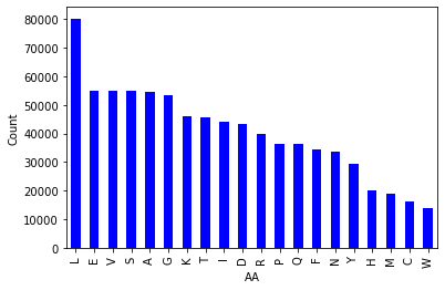
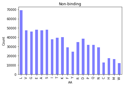
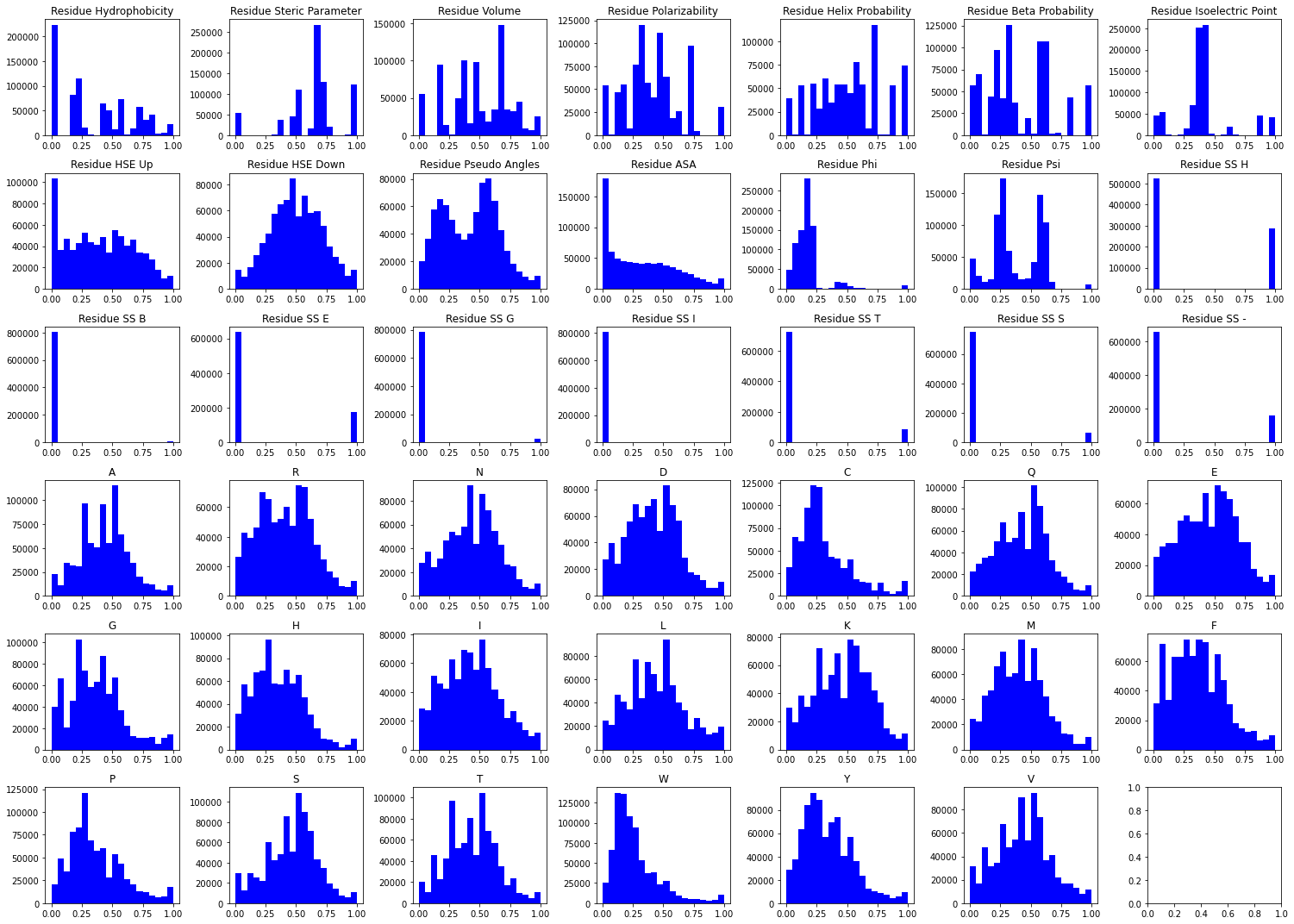
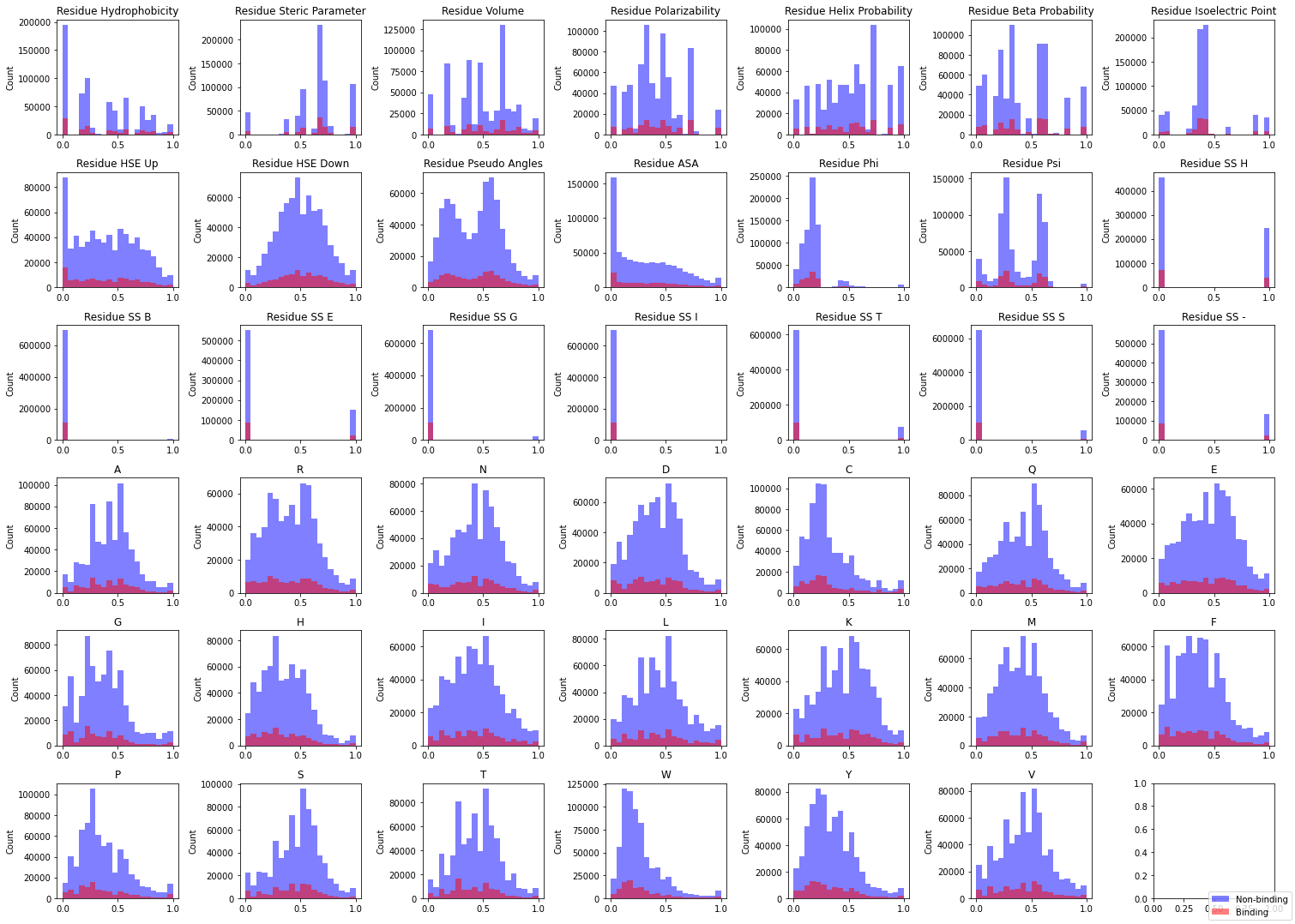
            "content_html": "<p><img src=\"https://cdn-images-1.medium.com/max/2864/0*Q27JiLau4SNxc5nZ.png\" alt=\"Visualization by Author\" /></p><p><a href=\"https://github.com/MurtoHilali/PepBDB-ML\"><img src=\"https://img.shields.io/badge/GitHub-View%20Repository-blue?style=round-square&amp;logo=github\" alt=\"GitHub Repo\" /></a><a href=\"https://github.com/MurtoHilali/PepBDB-ML/blob/main/LICENSE-CC\"><img src=\"https://img.shields.io/github/license/MurtoHilali/PepBDB-ML\" alt=\"License\" /></a><a href=\"https://github.com/MurtoHilali/PepBDB-ML/stargazers\"><img src=\"https://img.shields.io/github/stars/MurtoHilali/PepBDB-ML?style=social\" alt=\"Stars\" /></a></p><h2 id=\"table-of-contents\">Table of Contents</h2><ul>  <li><a href=\"#table-of-contents\">Table of Contents</a></li>  <li><a href=\"#background-cnns-can-predict-binding-sites\">Background: CNNs can predict binding sites</a></li>  <li><a href=\"#the-rationale-but-wait--does-the-data-really-matter-that-much\">The Rationale: But wait — does the data really matter that much?</a>    <ul>      <li><a href=\"#1-availability\">1. Availability</a></li>      <li><a href=\"#2-quality\">2. Quality</a></li>      <li><a href=\"#3-interpretability\">3. Interpretability</a></li>    </ul>  </li>  <li><a href=\"#the-process-building-the-pepbdb-ml-dataset\">The Process: Building the PepBDB-ML dataset</a></li>  <li><a href=\"#1-initial-filtering\">1. Initial filtering</a></li>  <li><a href=\"#2-sequence-extraction-using-biopython\">2. Sequence extraction using BioPython</a></li>  <li><a href=\"#3-binding-sequences-determination-with-prodigy\">3. Binding sequences determination with PRODIGY</a></li>  <li><a href=\"#4-adding-sequence-level-information-with-aaindex-and-psi-blast\">4. Adding sequence level information with AAindex and PSI-BLAST</a>    <ul>      <li><a href=\"#aaindex\">AAindex</a></li>      <li><a href=\"#psi-blast\">PSI-BLAST</a></li>    </ul>  </li>  <li><a href=\"#5-structural-information-using-biopython\">5. Structural information using BioPython</a>    <ul>      <li><a href=\"#secondary-structure-codes-half-sphere-exposure-and-from-dssp\">Secondary structure codes, half-sphere exposure, and from DSSP</a></li>    </ul>  </li>  <li><a href=\"#optional-generating-an-image-dataset\">Optional: Generating an image dataset</a></li>  <li><a href=\"#the-results-visualizing-the-pepbdb-ml-database\">The Results: Visualizing the PepBDB-ML database</a>    <ul>      <li><a href=\"#amino-acid-distributions\">Amino acid distributions</a></li>      <li><a href=\"#correlation-mapping\">Correlation mapping</a></li>      <li><a href=\"#feature-distributions\">Feature distributions</a></li>      <li><a href=\"#statistical-tests\">Statistical tests</a></li>    </ul>  </li>  <li><a href=\"#the-discussion-key-takeaways-and-learnings\">The Discussion: Key takeaways and learnings</a></li></ul><p>90% of the time I tell people I work with proteins, they assume I’m trying to get jacked.</p><p>And okay, fine, they’re right.</p><p>But really, I’m talking about <strong>biological proteins</strong>— incredible molecular machines that make it possible for your body to function.</p><p><img src=\"https://cdn-images-1.medium.com/max/13936/0*ib4VLHvLb-nWJjTA\" alt=\"Photo by [National Cancer Institute](https://unsplash.com/@nci?utm_source=medium&amp;utm_medium=referral) on [Unsplash](https://unsplash.com?utm_source=medium&amp;utm_medium=referral)\" /></p><p>Proteins are involved in <strong>vital metabolic processes</strong> — including getting that summer body — and <strong>peptide-protein interactions (PepPIs)</strong> are among the most important.</p><p>(Peptide = short protein segments).</p><p>Recently, I built a dataset I could use to study PepPIs. And by the end of this article, you will have too.</p><p><strong>Here’s a quick peek at a few things I discovered in what I’m calling the PepBDB-ML database:</strong></p><ul>  <li>    <p>Protein residue pseudo angles take on a bimodal distribution.</p>  </li>  <li>    <p>Substitution scores for residues are normally distributed (but there is one exception).</p>  </li>  <li>    <p>Amino acids that are typically found in beta sheets might be more open to swapping with isoleucine than other residues.</p>  </li></ul><p>But I’m getting ahead of myself —</p><p>Let’s start with some background.</p><h2 id=\"background-cnns-can-predict-binding-sites\">Background: CNNs can predict binding sites</h2><p>Recently, I read <a href=\"https://www.sciencedirect.com/science/article/pii/S0022519320301338?via%3Dihub\">a paper that used CNNs</a> to predict <strong>peptide-protein binding sites</strong> from a sequence.</p><ul>  <li>    <p>They took <strong>a context window from the sequence</strong> (7 amino acids, AKA residues), enriched it with data on hydrophobicity, exposure, relative angles, etc., and <strong>transformed it into an image.</strong></p>  </li>  <li>Repeating this across a body of residues created a massive dataset of training images.    <blockquote>      <p><em><strong>Analogy</strong>: Imagine you had a Lego Deathstar, and you took a picture of each brick — and these pictures were force-imbued, so you could see things like the age and weight of each brick. Label each image with data about where it goes in the Deathstar (e.g., interior vs exterior), and you’d learn how to classify new pieces.</em> <em>Protein = Deathstar, Lego brick = amino acid</em></p>    </blockquote>  </li>  <li>Feeding this into a <strong>CNN yielded a model with binding site detection rates twice as high</strong> as previously published methods.</li></ul><p><img src=\"https://cdn-images-1.medium.com/max/2000/0*nQ_R3fP2WysCt0Jk.jpg\" alt=\"From [Wardah et al.](https://www.sciencedirect.com/science/article/pii/S0022519320301338?via%3Dihub)\" /></p><p>I thought this approach was fascinating, but I saw an opportunity for improvement: residue secondary structure tags, angles, and accessible surface area were all predicted using SPIDER2 — <strong>but what if I just got the actual data from experimental structures instead?</strong></p><p>That’s precisely what I did using the PepBDB, a structural database of 3D peptide-receptor complexes (all structures are curated from the <a href=\"https://www.rcsb.org/pages/usage-policy\">RCSB PDB</a>, which provides data under license <a href=\"https://creativecommons.org/publicdomain/zero/1.0/\">CC0</a>).</p><p><img src=\"https://cdn-images-1.medium.com/max/4660/1*PBEv5SFgjEAvhMI2wyodRQ.png\" alt=\"Screenshot by Author, from [PepBDB](http://huanglab.phys.hust.edu.cn/pepbdb/db/1abo_C/)\" /></p><p>By using all the information applied in Visual, along with some structure-specific features, I could:</p><ul>  <li>    <p>Expand the dataset</p>  </li>  <li>    <p>Potentially improve model performance</p>  </li>  <li>    <p>Save the world</p>  </li></ul><p>(Two truths, one lie).</p><p>So that is precisely what I set out to do with <a href=\"https://github.com/MurtoHilali/PepBDB-ML\"><strong>PepBDB-ML</strong></a></p><h2 id=\"the-rationale-but-wait--does-the-data-really-matter-that-much\">The Rationale: But wait — does the data really matter that much?</h2><p>Well, there’s one key reason I think focusing on data is one of the highest-leverage activities in AI: <strong>data is our greatest constraint.</strong></p><p>Sure, compute is critical — but the data hydra has three heads:</p><h3 id=\"1-availability\">1. Availability</h3><p>Heard about the recent content licensing deal between OpenAI and News Corp, Vox Media, and The Atlantic? The agreement with News Corp alone is believed to be worth <a href=\"https://www.theverge.com/2024/5/29/24167072/openai-content-copyright-vox-media-the-atlantic\">over $250 million</a>.</p><p>While a lot of AI training data is either unprotected or open-source, <strong>the good stuff is often unavailable, expensive, or hard to find.</strong> Which leads to the next head…</p><h3 id=\"2-quality\">2. Quality</h3><p>Let’s use an example.</p><p>If LLMs right now are really good at generating text, why not use them to create more training data? Unfortunately, making AI eat its own tail causes something called <a href=\"https://www.bbva.ch/en/blog/innovacion/tecnologia/el-sindrome-de-la-vaca-loca-que-afecta-a-la-ia.html\">Model Autophagy Disorder</a>, or MAD — and yes, they came up with the acronym before deciding what it stood for.</p><p>Bottom line? Synthetic data can only take us so far. <strong>In the world of biology, that means we need reliable, experimental data</strong> (like the structures from PepBDB).</p><h3 id=\"3-interpretability\">3. Interpretability</h3><p>In biology specifically, human-readable data is often the most helpful. It allows us to unpack machine learning models and see things like:</p><ul>  <li>    <p>Critical features.</p>  </li>  <li>    <p>Relative importance.</p>  </li>  <li>    <p>The future (I’m only half-joking).</p>  </li></ul><p>For example, when it comes to peptide-protein binding, what’s more impactful — hydrophobicity or half-sphere exposure? Without labels, we can’t answer that question.</p><p><strong>Documented data means that models and humans can both learn more about biology.</strong></p><p><strong>Key Points:</strong></p><ul>  <li>    <p>We can always fine-tune ML/DL models, but <strong>we’re bottlenecked by the quality of our data</strong>.</p>  </li>  <li>    <p><strong>Availability, quality, and interpretability</strong> are crucial aspects of biological datasets.</p>  </li></ul><p>Now that you’re convinced we’re not wasting time, let’s get into the meat of this project: building the dataset.</p><h2 id=\"the-process-building-the-pepbdb-ml-dataset\">The Process: Building the PepBDB-ML dataset</h2><p>Before we begin, let’s decide what we want our dataset to <em>look</em> like.</p><ul>  <li>    <p><strong>A tabular version</strong>, where each row represents a residue from a protein complex and each column is a feature (like residue hydrophobicity, polarizability, secondary structure within the protein). These features will be the ones used in Visual, along with some extras.</p>  </li>  <li>    <p><strong>An image version</strong>, where each image is essentially 7 adjacent rows from the tabular dataset, representing a context window for the central amino acids.</p>  </li></ul><p>With this plan in mind, we can focus our efforts on the tabular dataset. Since the PepBDB database contains structures, we can use structural and sequence information. Here’s how we’ll approach this:</p><ol>  <li>    <p>Initial filtering</p>  </li>  <li>    <p>Sequence extraction + filtering</p>  </li>  <li>    <p>Binding residue determination with Prodigy</p>  </li>  <li>    <p>Sequence level information (AAindex, PSI-BLAST)</p>  </li>  <li>    <p>Structural information from BioPython (DSSP, HSE, Pseudo-angles)</p>  </li></ol><p>There’s going to be a lot of code coming up, <strong>so buckle up</strong>.</p><p>Before we begin, we’ll start with our imports:</p><div class=\"language-python highlighter-rouge\"><div class=\"highlight\"><pre class=\"highlight\"><code>    <span class=\"c1\"># gendata.py</span>        <span class=\"kn\">import</span> <span class=\"nn\">pandas</span> <span class=\"k\">as</span> <span class=\"n\">pd</span>    <span class=\"kn\">import</span> <span class=\"nn\">numpy</span> <span class=\"k\">as</span> <span class=\"n\">np</span>    <span class=\"kn\">import</span> <span class=\"nn\">argparse</span>    <span class=\"kn\">import</span> <span class=\"nn\">os</span>    <span class=\"kn\">import</span> <span class=\"nn\">pickle</span>        <span class=\"kn\">from</span> <span class=\"nn\">aaindex</span> <span class=\"kn\">import</span> <span class=\"o\">*</span>    <span class=\"kn\">from</span> <span class=\"nn\">helpers</span> <span class=\"kn\">import</span> <span class=\"o\">*</span>    <span class=\"kn\">from</span> <span class=\"nn\">paths</span> <span class=\"kn\">import</span> <span class=\"o\">*</span></code></pre></div></div><p>What are those ones at the bottom? Don’t worry — we’ll get to those soon.</p><p>(Heads up — since we’re going to be jumping between a few scripts, I’ll include the filename at the top of each code block).</p><h2 id=\"1-initial-filtering\">1. Initial filtering</h2><p>The PepBDB offers the peptidelist.txt file as part of its download. This file provides information about each peptide-protein pair in the repository.</p><div class=\"language-python highlighter-rouge\"><div class=\"highlight\"><pre class=\"highlight\"><code>    <span class=\"c1\"># gendata.py</span>        <span class=\"c1\">## Load the peptidelist.txt file</span>    <span class=\"n\">peptide_list</span> <span class=\"o\">=</span> <span class=\"n\">pd</span><span class=\"p\">.</span><span class=\"n\">read_csv</span><span class=\"p\">(</span><span class=\"n\">peptide_list_txt</span><span class=\"p\">,</span> <span class=\"n\">sep</span><span class=\"o\">=</span><span class=\"s\">'</span><span class=\"se\">\\\\\\\\</span><span class=\"s\">s+'</span><span class=\"p\">,</span> <span class=\"n\">header</span><span class=\"o\">=</span><span class=\"bp\">None</span><span class=\"p\">)</span>        <span class=\"n\">headers</span> <span class=\"o\">=</span> <span class=\"p\">[</span><span class=\"s\">'PDB ID'</span><span class=\"p\">,</span> <span class=\"s\">'Peptide Chain ID'</span><span class=\"p\">,</span> <span class=\"s\">'Peptide Length'</span><span class=\"p\">,</span> <span class=\"s\">'Number of Atoms in Peptide'</span><span class=\"p\">,</span>               <span class=\"s\">'Protein Chain ID'</span><span class=\"p\">,</span> <span class=\"s\">'Number of Atoms in Protein'</span><span class=\"p\">,</span>               <span class=\"s\">'Number of Atom Contacts'</span><span class=\"p\">,</span> <span class=\"s\">'unknown1'</span><span class=\"p\">,</span> <span class=\"s\">'unknown2'</span><span class=\"p\">,</span> <span class=\"s\">'Resolution'</span><span class=\"p\">,</span> <span class=\"s\">'Molecular Type'</span><span class=\"p\">]</span>    <span class=\"n\">peptide_list</span><span class=\"p\">.</span><span class=\"n\">columns</span> <span class=\"o\">=</span> <span class=\"n\">headers</span>        <span class=\"c1\"># 'pepbdb' below is the path to the PepBDB directory, imported from `paths`</span>    <span class=\"n\">peptide_list</span><span class=\"p\">[</span><span class=\"s\">'Peptide Path'</span><span class=\"p\">]</span> <span class=\"o\">=</span> <span class=\"n\">pepbdb</span> <span class=\"o\">+</span> <span class=\"n\">peptide_list</span><span class=\"p\">[</span><span class=\"s\">'PDB ID'</span><span class=\"p\">]</span> <span class=\"o\">+</span> <span class=\"s\">'_'</span> <span class=\"o\">+</span> <span class=\"n\">peptide_list</span><span class=\"p\">[</span><span class=\"s\">'Peptide Chain ID'</span><span class=\"p\">]</span> <span class=\"o\">+</span> <span class=\"s\">'/peptide.pdb'</span>    <span class=\"n\">peptide_list</span><span class=\"p\">[</span><span class=\"s\">'Protein Path'</span><span class=\"p\">]</span> <span class=\"o\">=</span> <span class=\"n\">pepbdb</span> <span class=\"o\">+</span> <span class=\"n\">peptide_list</span><span class=\"p\">[</span><span class=\"s\">'PDB ID'</span><span class=\"p\">]</span> <span class=\"o\">+</span> <span class=\"s\">'_'</span> <span class=\"o\">+</span> <span class=\"n\">peptide_list</span><span class=\"p\">[</span><span class=\"s\">'Peptide Chain ID'</span><span class=\"p\">]</span> <span class=\"o\">+</span> <span class=\"s\">'/receptor.pdb'</span>    <span class=\"n\">peptide_list</span><span class=\"p\">.</span><span class=\"n\">reset_index</span><span class=\"p\">(</span><span class=\"n\">drop</span><span class=\"o\">=</span><span class=\"bp\">True</span><span class=\"p\">)</span>        <span class=\"c1\">## Filter out nucleic acids, low-resolution, and small peptides</span>    <span class=\"n\">peptide_list</span> <span class=\"o\">=</span> <span class=\"n\">peptide_list</span><span class=\"p\">[</span><span class=\"n\">peptide_list</span><span class=\"p\">[</span><span class=\"s\">'Molecular Type'</span><span class=\"p\">]</span> <span class=\"o\">!=</span> <span class=\"s\">'prot-nuc'</span><span class=\"p\">]</span>    <span class=\"n\">peptide_list</span> <span class=\"o\">=</span> <span class=\"n\">peptide_list</span><span class=\"p\">[</span><span class=\"n\">peptide_list</span><span class=\"p\">[</span><span class=\"s\">'Resolution'</span><span class=\"p\">]</span> <span class=\"o\">&lt;</span> <span class=\"mf\">2.5</span><span class=\"p\">]</span>    <span class=\"n\">peptide_list</span> <span class=\"o\">=</span> <span class=\"n\">peptide_list</span><span class=\"p\">[</span><span class=\"n\">peptide_list</span><span class=\"p\">[</span><span class=\"s\">'Peptide Length'</span><span class=\"p\">]</span> <span class=\"o\">&gt;=</span> <span class=\"mi\">10</span><span class=\"p\">]</span>    <span class=\"k\">print</span><span class=\"p\">(</span><span class=\"s\">'</span><span class=\"se\">\\\\</span><span class=\"s\">033[1mInitial filtering done.</span><span class=\"se\">\\\\</span><span class=\"s\">033[0m'</span><span class=\"p\">)</span></code></pre></div></div><p>We’ll do some very simple filtering to begin:</p><ul>  <li>    <p><strong>Drop all prot-nuc models.</strong> These are models that contain a nucleic acid. We’re restricting this dataset to protein-only for the sake of simplicity.</p>  </li>  <li>    <p><strong>Drop models with resolution higher than 2.5 Å.</strong> We want our input data to be high-quality, so let’s drop any low-res models.</p>  </li>  <li>    <p><strong>Drop models with extra short peptides.</strong> This is mainly for the sake of computational efficiency. We’ll drop any peptides shorter than ten amino acids.</p>  </li></ul><p>In the next step, <strong>we’ll use BioPython to extract the sequences</strong> from each of our remaining models. Sequence extraction can take some time, which is why I’ve chosen to do it after some initial cleanup.</p><h2 id=\"2-sequence-extraction-using-biopython\">2. Sequence extraction using BioPython</h2><p>PepBDB provides 3D models but not direct sequences. Fortunately, these are relatively simple to extract using BioPython.</p><p>To keep the code clean, I’ll create a helper function in a separate file called helpers.py:</p><div class=\"language-python highlighter-rouge\"><div class=\"highlight\"><pre class=\"highlight\"><code>    <span class=\"c1\"># helpers.py</span>        <span class=\"k\">def</span> <span class=\"nf\">extract_sequence</span><span class=\"p\">(</span><span class=\"n\">pdb_filename</span><span class=\"p\">:</span> <span class=\"nb\">str</span><span class=\"p\">)</span> <span class=\"o\">-&gt;</span> <span class=\"nb\">str</span><span class=\"p\">:</span>        <span class=\"s\">'''        Helper function that extracts the sequence from a PDB file.        '''</span>        <span class=\"n\">parser</span> <span class=\"o\">=</span> <span class=\"n\">PDBParser</span><span class=\"p\">()</span>        <span class=\"n\">structure</span> <span class=\"o\">=</span> <span class=\"n\">parser</span><span class=\"p\">.</span><span class=\"n\">get_structure</span><span class=\"p\">(</span><span class=\"s\">'X'</span><span class=\"p\">,</span> <span class=\"n\">pdb_filename</span><span class=\"p\">)</span>                <span class=\"n\">sequence</span> <span class=\"o\">=</span> <span class=\"s\">''</span>        <span class=\"n\">contains_unk</span> <span class=\"o\">=</span> <span class=\"bp\">False</span>                <span class=\"k\">for</span> <span class=\"n\">model</span> <span class=\"ow\">in</span> <span class=\"n\">structure</span><span class=\"p\">:</span>            <span class=\"k\">for</span> <span class=\"n\">chain</span> <span class=\"ow\">in</span> <span class=\"n\">model</span><span class=\"p\">:</span>                <span class=\"n\">residues</span> <span class=\"o\">=</span> <span class=\"n\">chain</span><span class=\"p\">.</span><span class=\"n\">get_residues</span><span class=\"p\">()</span>                <span class=\"k\">for</span> <span class=\"n\">residue</span> <span class=\"ow\">in</span> <span class=\"n\">residues</span><span class=\"p\">:</span>                    <span class=\"k\">if</span> <span class=\"n\">residue</span><span class=\"p\">.</span><span class=\"n\">get_resname</span><span class=\"p\">()</span> <span class=\"o\">==</span> <span class=\"s\">'HOH'</span><span class=\"p\">:</span> <span class=\"c1\"># ignoring water</span>                        <span class=\"k\">continue</span>                    <span class=\"k\">if</span> <span class=\"n\">residue</span><span class=\"p\">.</span><span class=\"n\">get_resname</span><span class=\"p\">()</span> <span class=\"o\">==</span> <span class=\"s\">'UNK'</span><span class=\"p\">:</span>                        <span class=\"n\">sequence</span> <span class=\"o\">+=</span> <span class=\"s\">'X'</span>  <span class=\"c1\"># add X for each 'UNK' residue</span>                    <span class=\"k\">else</span><span class=\"p\">:</span>                        <span class=\"n\">sequence</span> <span class=\"o\">+=</span> <span class=\"n\">seq1</span><span class=\"p\">(</span><span class=\"n\">residue</span><span class=\"p\">.</span><span class=\"n\">get_resname</span><span class=\"p\">())</span> <span class=\"c1\"># seq1 converts 3-letter code to 1-letter code</span>            <span class=\"k\">return</span> <span class=\"n\">sequence</span></code></pre></div></div><p>Then, I’ll import it into our data generation script and apply it to our dataset:</p><div class=\"language-python highlighter-rouge\"><div class=\"highlight\"><pre class=\"highlight\"><code>    <span class=\"c1\"># gendata.py</span>        <span class=\"n\">peptide_list</span><span class=\"p\">[</span><span class=\"s\">'Peptide Sequence'</span><span class=\"p\">]</span> <span class=\"o\">=</span> <span class=\"n\">peptide_list</span><span class=\"p\">[</span><span class=\"s\">'Peptide Path'</span><span class=\"p\">].</span><span class=\"nb\">apply</span><span class=\"p\">(</span><span class=\"n\">extract_sequence</span><span class=\"p\">)</span>    <span class=\"n\">peptide_list</span><span class=\"p\">[</span><span class=\"s\">'Protein Sequence'</span><span class=\"p\">]</span> <span class=\"o\">=</span> <span class=\"n\">peptide_list</span><span class=\"p\">[</span><span class=\"s\">'Protein Path'</span><span class=\"p\">].</span><span class=\"nb\">apply</span><span class=\"p\">(</span><span class=\"n\">extract_sequence</span><span class=\"p\">)</span>        <span class=\"k\">print</span><span class=\"p\">(</span><span class=\"s\">'</span><span class=\"se\">\\\\\\\\</span><span class=\"s\">033[1mSequences extracted.</span><span class=\"se\">\\\\\\\\</span><span class=\"s\">033[0m'</span><span class=\"p\">)</span></code></pre></div></div><p>Now that we have sequences for each PDB structure, let’s remove the problematic ones (sequences with non-standard amino acids):</p><div class=\"language-python highlighter-rouge\"><div class=\"highlight\"><pre class=\"highlight\"><code>    <span class=\"c1\"># gendata.py</span>        <span class=\"n\">peptide_list</span> <span class=\"o\">=</span> <span class=\"n\">peptide_list</span><span class=\"p\">[</span><span class=\"o\">~</span><span class=\"n\">peptide_list</span><span class=\"p\">[</span><span class=\"s\">'Peptide Sequence'</span><span class=\"p\">].</span><span class=\"nb\">str</span><span class=\"p\">.</span><span class=\"n\">contains</span><span class=\"p\">(</span><span class=\"s\">'[UOBZJX</span><span class=\"se\">\\\\\\\\\\\\\\\\</span><span class=\"s\">*]'</span><span class=\"p\">,</span> <span class=\"n\">regex</span><span class=\"o\">=</span><span class=\"bp\">True</span><span class=\"p\">)]</span>    <span class=\"n\">peptide_list</span> <span class=\"o\">=</span> <span class=\"n\">peptide_list</span><span class=\"p\">[</span><span class=\"o\">~</span><span class=\"n\">peptide_list</span><span class=\"p\">[</span><span class=\"s\">'Protein Sequence'</span><span class=\"p\">].</span><span class=\"nb\">str</span><span class=\"p\">.</span><span class=\"n\">contains</span><span class=\"p\">(</span><span class=\"s\">'[UOBZJX</span><span class=\"se\">\\\\\\\\\\\\\\\\</span><span class=\"s\">*]'</span><span class=\"p\">,</span> <span class=\"n\">regex</span><span class=\"o\">=</span><span class=\"bp\">True</span><span class=\"p\">)]</span>        <span class=\"n\">peptide_list</span> <span class=\"o\">=</span> <span class=\"n\">peptide_list</span><span class=\"p\">.</span><span class=\"n\">drop_duplicates</span><span class=\"p\">(</span><span class=\"n\">subset</span><span class=\"o\">=</span><span class=\"p\">[</span><span class=\"s\">'Peptide Sequence'</span><span class=\"p\">,</span> <span class=\"s\">'Protein Sequence'</span><span class=\"p\">])</span></code></pre></div></div><p><img src=\"https://cdn-images-1.medium.com/max/3736/1*NbNPHXAj8wuAM3QERvJdPQ.png\" alt=\"Screenshot by Author\" /></p><h2 id=\"3-binding-sequences-determination-with-prodigy\">3. Binding sequences determination with PRODIGY</h2><p><a href=\"https://github.com/haddocking/prodigy\">PRODIGY</a> (PROtein binDIng enerGY prediction) is <strong>a tool for predicting binding affinities</strong> for protein structures from 3D data.</p><p>Part of that involves <strong>identifying residues in contact with each other — i.e., involved in binding.</strong></p><p>I used PRODIGY on every PDB in the PepBDB leftover from the last preprocessing step. The program outputs a .icfile — a simple text file that lists the residues involved in binding.</p><p>Here’s an example for <a href=\"https://www.rcsb.org/structure/1A03\">calcium-bound cyclin</a> (1A03):</p><pre><code class=\"language-plain\">      GLY    78   A   GLN    71   B      ILE    13   A   TYR    84   B      LYS    40   A   MET     1   B      GLU    86   A   HIS    27   B      LEU    88   A   LEU    12   B      ALA     8   A   ILE    15   B      MET     1   A   LYS    40   B      ALA    87   A   ILE    13   B      PHE    70   A   LEU    77   B      GLN    71   A   MET    82   B      ALA     8   A   ALA     8   B      ILE    74   A   LEU    77   B      LYS    89   A   LYS    26   B</code></pre><p>Processing this data gives us two lists of indices, each referring to a binding residue.</p><p>The peptides and receptors in each row are available as distinct PDBs, i.e. their models contain one chain each. For our purposes, PRODIGY needs a complex (2 chains), so we’ll make a temporary file and process the output:</p><div class=\"language-python highlighter-rouge\"><div class=\"highlight\"><pre class=\"highlight\"><code>    <span class=\"c1\"># helpers.py</span>        <span class=\"k\">def</span> <span class=\"nf\">label_residues</span><span class=\"p\">(</span><span class=\"n\">peptide_path</span><span class=\"p\">:</span> <span class=\"nb\">str</span><span class=\"p\">,</span> <span class=\"n\">protein_path</span><span class=\"p\">:</span> <span class=\"nb\">str</span><span class=\"p\">)</span> <span class=\"o\">-&gt;</span> <span class=\"n\">List</span><span class=\"p\">:</span>        <span class=\"c1\"># creating a temporary file with the peptide and protein</span>        <span class=\"k\">with</span> <span class=\"n\">tempfile</span><span class=\"p\">.</span><span class=\"n\">NamedTemporaryFile</span><span class=\"p\">(</span><span class=\"n\">suffix</span><span class=\"o\">=</span><span class=\"s\">'.pdb'</span><span class=\"p\">,</span> <span class=\"n\">delete</span><span class=\"o\">=</span><span class=\"bp\">False</span><span class=\"p\">)</span> <span class=\"k\">as</span> <span class=\"n\">temp_file</span><span class=\"p\">:</span>            <span class=\"n\">output_path</span> <span class=\"o\">=</span> <span class=\"n\">temp_file</span><span class=\"p\">.</span><span class=\"n\">name</span>            <span class=\"n\">subprocess</span><span class=\"p\">.</span><span class=\"n\">run</span><span class=\"p\">([</span><span class=\"s\">'cat'</span><span class=\"p\">,</span> <span class=\"n\">peptide_path</span><span class=\"p\">,</span> <span class=\"n\">protein_path</span><span class=\"p\">],</span> <span class=\"n\">stdout</span><span class=\"o\">=</span><span class=\"n\">temp_file</span><span class=\"p\">)</span>            <span class=\"c1\"># ensuring the temp file is properly closed before using it in subprocess</span>        <span class=\"n\">temp_file</span><span class=\"p\">.</span><span class=\"n\">close</span><span class=\"p\">()</span>                <span class=\"c1\"># obtaining binding residues using PRODIGY</span>        <span class=\"k\">try</span><span class=\"p\">:</span>            <span class=\"n\">subprocess</span><span class=\"p\">.</span><span class=\"n\">run</span><span class=\"p\">([</span><span class=\"s\">'prodigy'</span><span class=\"p\">,</span> <span class=\"s\">'-q'</span><span class=\"p\">,</span> <span class=\"s\">'--contact_list'</span><span class=\"p\">,</span> <span class=\"n\">output_path</span><span class=\"p\">],</span> <span class=\"n\">check</span><span class=\"o\">=</span><span class=\"bp\">True</span><span class=\"p\">)</span>        <span class=\"k\">except</span> <span class=\"n\">subprocess</span><span class=\"p\">.</span><span class=\"n\">CalledProcessError</span> <span class=\"k\">as</span> <span class=\"n\">e</span><span class=\"p\">:</span>            <span class=\"k\">print</span><span class=\"p\">(</span><span class=\"sa\">f</span><span class=\"s\">\"An error occurred while processing the files: </span><span class=\"si\">{</span><span class=\"n\">peptide_path</span><span class=\"si\">}</span><span class=\"s\"> &amp; </span><span class=\"si\">{</span><span class=\"n\">protein_path</span><span class=\"si\">}</span><span class=\"s\">\"</span><span class=\"p\">)</span>            <span class=\"k\">print</span><span class=\"p\">(</span><span class=\"sa\">f</span><span class=\"s\">\"Error: </span><span class=\"si\">{</span><span class=\"n\">e</span><span class=\"si\">}</span><span class=\"s\">\"</span><span class=\"p\">)</span>                <span class=\"c1\"># the .ic file will have the same root name as the input file</span>        <span class=\"n\">ic_file_path</span> <span class=\"o\">=</span> <span class=\"n\">output_path</span><span class=\"p\">.</span><span class=\"n\">replace</span><span class=\"p\">(</span><span class=\"s\">'.pdb'</span><span class=\"p\">,</span> <span class=\"s\">'.ic'</span><span class=\"p\">)</span>            <span class=\"c1\"># check if the .ic file exists before reading</span>        <span class=\"k\">if</span> <span class=\"ow\">not</span> <span class=\"n\">os</span><span class=\"p\">.</span><span class=\"n\">path</span><span class=\"p\">.</span><span class=\"n\">exists</span><span class=\"p\">(</span><span class=\"n\">ic_file_path</span><span class=\"p\">):</span>            <span class=\"k\">raise</span> <span class=\"nb\">FileNotFoundError</span><span class=\"p\">(</span><span class=\"sa\">f</span><span class=\"s\">\"</span><span class=\"si\">{</span><span class=\"n\">ic_file_path</span><span class=\"si\">}</span><span class=\"s\"> not found after running PRODIGY.\"</span><span class=\"p\">)</span>                <span class=\"c1\"># are you actually reading these comments? kudos! if yes — reply with a 😼</span>        <span class=\"n\">contacts</span> <span class=\"o\">=</span> <span class=\"n\">pd</span><span class=\"p\">.</span><span class=\"n\">read_csv</span><span class=\"p\">(</span><span class=\"n\">ic_file_path</span><span class=\"p\">,</span> <span class=\"n\">sep</span><span class=\"o\">=</span><span class=\"s\">'\\s+'</span><span class=\"p\">,</span> <span class=\"n\">header</span><span class=\"o\">=</span><span class=\"bp\">None</span><span class=\"p\">)</span>        <span class=\"n\">contacts</span><span class=\"p\">.</span><span class=\"n\">columns</span> <span class=\"o\">=</span> <span class=\"p\">[</span><span class=\"s\">'peptide_residue'</span><span class=\"p\">,</span> <span class=\"s\">'peptide_index'</span><span class=\"p\">,</span> <span class=\"s\">'peptide_chain'</span><span class=\"p\">,</span> <span class=\"s\">'protein_residue'</span><span class=\"p\">,</span> <span class=\"s\">'protein_index'</span><span class=\"p\">,</span> <span class=\"s\">'protein_chain'</span><span class=\"p\">]</span>                <span class=\"n\">peptide_binding_residues</span> <span class=\"o\">=</span> <span class=\"nb\">sorted</span><span class=\"p\">(</span><span class=\"nb\">list</span><span class=\"p\">(</span><span class=\"n\">contacts</span><span class=\"p\">[</span><span class=\"s\">'peptide_index'</span><span class=\"p\">].</span><span class=\"n\">unique</span><span class=\"p\">()))</span>        <span class=\"n\">protein_binding_residues</span> <span class=\"o\">=</span> <span class=\"nb\">sorted</span><span class=\"p\">(</span><span class=\"nb\">list</span><span class=\"p\">(</span><span class=\"n\">contacts</span><span class=\"p\">[</span><span class=\"s\">'protein_index'</span><span class=\"p\">].</span><span class=\"n\">unique</span><span class=\"p\">()))</span>                <span class=\"n\">os</span><span class=\"p\">.</span><span class=\"n\">remove</span><span class=\"p\">(</span><span class=\"n\">output_path</span><span class=\"p\">)</span>                <span class=\"k\">return</span> <span class=\"n\">peptide_binding_residues</span><span class=\"p\">,</span> <span class=\"n\">protein_binding_residues</span></code></pre></div></div><p>Now, let’s apply it to our dataset:</p><div class=\"language-python highlighter-rouge\"><div class=\"highlight\"><pre class=\"highlight\"><code>    <span class=\"c1\"># gendata.py</span>        <span class=\"k\">print</span><span class=\"p\">(</span><span class=\"s\">'Running PRODIGY to determine binding contacts...'</span><span class=\"p\">)</span>        <span class=\"c1\">## determine binding residues from peptide-protein complexes</span>    <span class=\"n\">peptide_list</span><span class=\"p\">[</span><span class=\"s\">'Peptide Binding Indices'</span><span class=\"p\">]</span> <span class=\"o\">=</span> <span class=\"n\">np</span><span class=\"p\">.</span><span class=\"n\">nan</span>    <span class=\"n\">peptide_list</span><span class=\"p\">[</span><span class=\"s\">'Protein Binding Indices'</span><span class=\"p\">]</span> <span class=\"o\">=</span> <span class=\"n\">np</span><span class=\"p\">.</span><span class=\"n\">nan</span>        <span class=\"k\">for</span> <span class=\"n\">index</span><span class=\"p\">,</span> <span class=\"n\">row</span> <span class=\"ow\">in</span> <span class=\"n\">peptide_list</span><span class=\"p\">.</span><span class=\"n\">iterrows</span><span class=\"p\">():</span>        <span class=\"n\">peptide_path</span> <span class=\"o\">=</span> <span class=\"n\">row</span><span class=\"p\">[</span><span class=\"s\">'Peptide Path'</span><span class=\"p\">]</span>        <span class=\"n\">protein_path</span> <span class=\"o\">=</span> <span class=\"n\">row</span><span class=\"p\">[</span><span class=\"s\">'Protein Path'</span><span class=\"p\">]</span>        <span class=\"n\">peptide_binding_positions</span><span class=\"p\">,</span> <span class=\"n\">protein_binding_positions</span> <span class=\"o\">=</span> <span class=\"n\">label_residues</span><span class=\"p\">(</span><span class=\"n\">peptide_path</span><span class=\"p\">,</span> <span class=\"n\">protein_path</span><span class=\"p\">)</span>        <span class=\"n\">peptide_list</span><span class=\"p\">.</span><span class=\"n\">at</span><span class=\"p\">[</span><span class=\"n\">index</span><span class=\"p\">,</span> <span class=\"s\">'Peptide Binding Indices'</span><span class=\"p\">]</span> <span class=\"o\">=</span> <span class=\"nb\">str</span><span class=\"p\">(</span><span class=\"n\">peptide_binding_positions</span><span class=\"p\">)</span>        <span class=\"n\">peptide_list</span><span class=\"p\">.</span><span class=\"n\">at</span><span class=\"p\">[</span><span class=\"n\">index</span><span class=\"p\">,</span> <span class=\"s\">'Protein Binding Indices'</span><span class=\"p\">]</span> <span class=\"o\">=</span> <span class=\"nb\">str</span><span class=\"p\">(</span><span class=\"n\">protein_binding_positions</span><span class=\"p\">)</span>    <span class=\"k\">print</span><span class=\"p\">(</span><span class=\"s\">'</span><span class=\"se\">\\\\\\\\</span><span class=\"s\">033[1mBinding indices identified.</span><span class=\"se\">\\\\\\\\</span><span class=\"s\">033[0m'</span><span class=\"p\">)</span></code></pre></div></div><p><img src=\"https://cdn-images-1.medium.com/max/3816/1*-xkLotcf_ODC4K0UikYA3g.png\" alt=\"Screenshot by Author\" /></p><blockquote>  <p>The Biology: <em>You might be wondering — why build this dataset if we can use PRODIGY to get binding sites? Well, PRODIGY generally needs two chains in complex. Our dataset is aimed at helping ML/DL models predict binding sites with just one model chain.</em></p></blockquote><h2 id=\"4-adding-sequence-level-information-with-aaindex-and-psi-blast\">4. Adding sequence level information with AAindex and PSI-BLAST</h2><h3 id=\"aaindex\"><a href=\"https://academic.oup.com/nar/article/28/1/374/2384334\">AAindex</a></h3><p>We’ve now got a list of protein sequences. We can enrich our dataset by adding publically available, residue-specific information from the <a href=\"https://www.genome.jp/aaindex/\">Amino Acid Index Database</a> — a cornucopia of known, reference amino acid features.</p><p>For example, here’s hydrophobicity:</p><pre><code class=\"language-plain\">    H ARGP820101    D Hydrophobicity index (Argos et al., 1982)    R PMID:7151796    A Argos, P., Rao, J.K.M. and Hargrave, P.A.    T Structural prediction of membrane-bound proteins    J Eur. J. Biochem. 128, 565-575 (1982)    C JOND750101    1.000  SIMZ760101    0.967  GOLD730101    0.936      TAKK010101    0.906  MEEJ810101    0.891  ROSM880104    0.872      CIDH920105    0.867  LEVM760106    0.865  CIDH920102    0.862      MEEJ800102    0.855  MEEJ810102    0.853  ZHOH040101    0.841      CIDH920103    0.827  PLIV810101    0.820  CIDH920104    0.819      LEVM760107    0.806  NOZY710101    0.800  GUYH850103   -0.808      PARJ860101   -0.835  WOLS870101   -0.838  BULH740101   -0.854    I    A/L     R/K     N/M     D/F     C/P     Q/S     E/T     G/W     H/Y     I/V        0.61    0.60    0.06    0.46    1.07      0.    0.47    0.07    0.61    2.22        1.53    1.15    1.18    2.02    1.95    0.05    0.05    2.65    1.88    1.32    //</code></pre><p>We’re interested in those values along the bottom. These are the feature Infinity Stones I collected for our dataset Gauntlet:</p><ul>  <li><strong><a href=\"https://www.jbc.org/article/S0021-9258(19)77210-X/pdf\">Hydrophobicity</a></strong>: a measure of the tendency of that side chain to be located in the interior of a native protein molecule. Normalized to be unitless.    <blockquote>      <p>Note: <em>In the original paper, the units were ΔFₜ — for the transfer of the amino acid side chain from organic solvent to water at 25° in cal/mole. Here, they are all made positive and normalized to a value of 1.0, which means they adjusted the scale so that the average value is 1.0.</em></p>    </blockquote>  </li>  <li>    <p><strong><a href=\"https://www.sciencedirect.com/science/article/pii/0022519381903775?via%3Dihub\">Steric parameter</a></strong>: the tendency of amino acids to be found at the surface of globular proteins as a function of side-chain structure. Unitless, but calculated based on van der Waals radii.</p>  </li>  <li>    <p><strong><a href=\"https://www.sciencedirect.com/science/article/pii/0022519367900045?via%3Dihub\">Residue volume</a></strong>: The space a residue occupies. Units are Å².</p>  </li>  <li>    <p><strong><a href=\"https://www.sciencedirect.com/science/article/pii/0022519382901916\">Polarizability</a></strong>: a measure of how easily an amino acid’s electron cloud will form dipoles in response to external forces. Unitless, a relative measure.</p>  </li>  <li>    <p><strong><a href=\"https://onlinelibrary.wiley.com/doi/10.1002/bip.1980.360190906\">Average relative probability of helix</a></strong>: the relative helix residue probability in 47 proteins. Unitless, relative measure.</p>  </li>  <li>    <p><strong><a href=\"https://onlinelibrary.wiley.com/doi/10.1002/bip.1980.360190906\">Average relative probability of beta sheet</a></strong>: the relative beta sheet residue probability in 47 proteins. It is also a unitless, relative measure.</p>  </li>  <li><strong><a href=\"https://www.sciencedirect.com/science/article/pii/0022519368900696\">Isoelectric point</a></strong>: the pH at which an amino acid is electrically neutral. Units are pH.    <blockquote>      <p>The Biology: <em>Why these features? Here’s an example: we might expect binding residues to be on the surface of the protein, where it can easily bind to other peptides — so a measure like steric parameter is useful.</em></p>    </blockquote>  </li></ul><p>Using AAindex1, I load all of these indices into a script aaindex.py full of dictionaries and a function to access them:</p><div class=\"language-python highlighter-rouge\"><div class=\"highlight\"><pre class=\"highlight\"><code>    <span class=\"c1\"># aaindex.py</span>        <span class=\"k\">def</span> <span class=\"nf\">feature_vector</span><span class=\"p\">(</span><span class=\"n\">seq</span><span class=\"p\">:</span> <span class=\"nb\">str</span><span class=\"p\">,</span> <span class=\"n\">feature_type</span><span class=\"p\">:</span> <span class=\"nb\">dict</span><span class=\"p\">):</span>        <span class=\"s\">'''        Returns a list of feature values corresponding to each        residue in sequence, according to AAindex1.                Feature types include:        - Hydrophobicity        - Steric parameter        - Residue volume        - Polarizability        - Average relative probability of helix        - Average relative probability of beta        - Isoelectric point        '''</span>        <span class=\"k\">return</span> <span class=\"p\">[</span><span class=\"n\">feature_type</span><span class=\"p\">[</span><span class=\"n\">aa</span><span class=\"p\">]</span> <span class=\"k\">for</span> <span class=\"n\">aa</span> <span class=\"ow\">in</span> <span class=\"n\">seq</span><span class=\"p\">]</span>        <span class=\"n\">hydrophobicity</span> <span class=\"o\">=</span> <span class=\"p\">{</span>        <span class=\"s\">'A'</span><span class=\"p\">:</span> <span class=\"mf\">0.61</span><span class=\"p\">,</span>      <span class=\"p\">...,</span>        <span class=\"s\">'V'</span><span class=\"p\">:</span> <span class=\"mf\">1.32</span>    <span class=\"p\">}</span></code></pre></div></div><p>Next, I extract this information from every sequence:</p><div class=\"language-python highlighter-rouge\"><div class=\"highlight\"><pre class=\"highlight\"><code>    <span class=\"c1\"># gendata.py</span>        <span class=\"k\">print</span><span class=\"p\">(</span><span class=\"s\">'Adding residue-level data from AAindex1...'</span><span class=\"p\">)</span>        <span class=\"c1\">## Add rich data from AAindex1</span>    <span class=\"n\">features</span> <span class=\"o\">=</span> <span class=\"p\">{</span>     <span class=\"s\">'Hydrophobicity'</span><span class=\"p\">:</span> <span class=\"n\">hydrophobicity</span><span class=\"p\">,</span>      <span class=\"s\">'Steric Parameter'</span><span class=\"p\">:</span> <span class=\"n\">steric_parameter</span><span class=\"p\">,</span>      <span class=\"s\">'Volume'</span><span class=\"p\">:</span> <span class=\"n\">residue_volume</span><span class=\"p\">,</span>      <span class=\"s\">'Polarizability'</span><span class=\"p\">:</span> <span class=\"n\">polarizability</span><span class=\"p\">,</span>      <span class=\"s\">'Helix Probability'</span><span class=\"p\">:</span> <span class=\"n\">average_relative_probability_of_helix</span><span class=\"p\">,</span>      <span class=\"s\">'Beta Probability'</span><span class=\"p\">:</span> <span class=\"n\">average_relative_probability_of_beta_sheet</span><span class=\"p\">,</span>      <span class=\"s\">'Isoelectric Point'</span><span class=\"p\">:</span> <span class=\"n\">isoelectric_point</span>        <span class=\"p\">}</span>    <span class=\"k\">for</span> <span class=\"n\">feature_name</span><span class=\"p\">,</span> <span class=\"n\">feature_function</span> <span class=\"ow\">in</span> <span class=\"n\">features</span><span class=\"p\">.</span><span class=\"n\">items</span><span class=\"p\">():</span>     <span class=\"n\">peptide_list</span><span class=\"p\">[</span><span class=\"sa\">f</span><span class=\"s\">'Peptide </span><span class=\"si\">{</span><span class=\"n\">feature_name</span><span class=\"si\">}</span><span class=\"s\">'</span><span class=\"p\">]</span> <span class=\"o\">=</span> <span class=\"n\">peptide_list</span><span class=\"p\">[</span><span class=\"s\">'Peptide Sequence'</span><span class=\"p\">].</span><span class=\"nb\">apply</span><span class=\"p\">(</span><span class=\"k\">lambda</span> <span class=\"n\">x</span><span class=\"p\">:</span> <span class=\"n\">feature_vector</span><span class=\"p\">(</span><span class=\"n\">x</span><span class=\"p\">,</span> <span class=\"n\">feature_function</span><span class=\"p\">))</span>      <span class=\"n\">peptide_list</span><span class=\"p\">[</span><span class=\"sa\">f</span><span class=\"s\">'Protein </span><span class=\"si\">{</span><span class=\"n\">feature_name</span><span class=\"si\">}</span><span class=\"s\">'</span><span class=\"p\">]</span> <span class=\"o\">=</span> <span class=\"n\">peptide_list</span><span class=\"p\">[</span><span class=\"s\">'Protein Sequence'</span><span class=\"p\">].</span><span class=\"nb\">apply</span><span class=\"p\">(</span><span class=\"k\">lambda</span> <span class=\"n\">x</span><span class=\"p\">:</span> <span class=\"n\">feature_vector</span><span class=\"p\">(</span><span class=\"n\">x</span><span class=\"p\">,</span> <span class=\"n\">feature_function</span><span class=\"p\">))</span>    <span class=\"k\">print</span><span class=\"p\">(</span><span class=\"s\">'</span><span class=\"se\">\\\\</span><span class=\"s\">033[1mAAindex features added.</span><span class=\"se\">\\\\</span><span class=\"s\">033[0m'</span><span class=\"p\">)</span></code></pre></div></div><p><img src=\"https://cdn-images-1.medium.com/max/3832/1*ejHMdcHkbdFly-i9YkZSPw.png\" alt=\"Screenshot by Author\" /></p><p>Note: <em>since completing this piece, I’ve discovered a <a href=\"https://github.com/amckenna41/aaindex\">Python package</a> for accessing all data from the AAindex. Which means I didn’t need to write this script from scratch. Yes, I have feelings about this. No, I will not be discussing them.</em></p><h3 id=\"psi-blast\">PSI-BLAST</h3><p>Next, let’s use PSI-BLAST to get residue-level conservation scores.</p><p><a href=\"https://www.ncbi.nlm.nih.gov/pmc/articles/PMC4781153/\">PSI-BLAST</a> (Position-Specific Iterative Basic Local Alignment Search Tool) is a sequence alignment tool that lets us build a <strong>Position Specific Scoring Matrix (PSSM)</strong> from a sequence.</p><p><strong>A PSSM tells us how conserved a given residue is at a given position</strong> in the sequence. High score = highly conserved.</p><blockquote>  <p>The Biology: <em>Why do we want this information? Binding motifs are typically highly conserved — alterations could mean loss of binding function, stymying organism survival.</em></p></blockquote><p>Here’s an example for the same protein we looked at earlier, 1A03:</p><div class=\"language-plaintext highlighter-rouge\"><div class=\"highlight\"><pre class=\"highlight\"><code>    Last position-specific scoring matrix computed, weighted observed percentages rounded down, information per position, and relative weight of gapless real matches to pseudocounts                A   R   N   D   C   Q   E   G   H   I   L   K   M   F   P   S   T   W   Y   V   A   R   N   D   C   Q   E   G   H   I   L   K   M   F   P   S   T   W   Y   V        1 M    -3  -4  -4  -5  -4  -3  -4  -5  -4  -1   0  -4  10  -2  -5  -4  -3  -4  -3  -1    0   0   0   0   0   0   0   0   0   0   0   0 100   0   0   0   0   0   0   0  2.17 0.45        2 A     1  -3   0  -2   1  -2  -1   1  -3  -3  -2  -2  -3  -4   6   0  -1  -4  -4  -3   14   0   5   0   4   0   3  12   0   0   5   0   0   0  48   7   2   0   0   0  0.92 0.21        3 S    -1   0  -1  -2   1  -2  -2  -2  -2  -1  -3  -1  -2  -3  -2   4   4  -4  -3  -2    2   6   0   1   3   0   1   1   0   4   1   2   0   0   0  40  37   0   0   1  0.61 0.25        4 P    -2  -2  -2   3  -5   4   3  -3  -2  -4  -3   1  -3  -5   4  -1  -2  -5  -4  -4    0   0   0  15   0  23  22   0   0   0   3   9   0   0  25   1   0   0   0   0  0.80 0.28                                                ....       86 E    -2  -1   0   3  -4   0   4  -3   2  -3  -2   3  -3  -4   0  -2  -2  -4  -1  -3    0   0   3  20   0   0  33   0   5   1   5  26   0   0   5   0   0   0   2   0  0.55 0.20       87 A    -1  -1   0   0  -3   2   0  -3   2  -1  -2   2  -2   3  -3   0  -1  -1   3  -1    4   0   3   6   0  11   5   0   6   4   0  17   0  14   0   9   0   0  15   6  0.21 0.12       88 L    -2  -3  -3  -4  -3  -3  -4  -4  -3   1   3  -3   3   5  -4   1  -1  -1   2  -1    0   0   0   0   0   0   0   0   0   7  28   0   9  34   0  14   2   0   6   0  0.54 0.19       89 K    -3   0  -1   0  -5   2   2  -3   9  -5  -4   2  -3  -3  -3  -2  -3  -4   0  -4    0   2   0   5   0   7  11   0  62   0   0  12   0   0   0   0   0   0   0   0  1.18 0.25       90 G     0  -2   3  -1  -3  -2  -2   5  -2  -4  -4  -2  -3  -4  -3   0  -2  -3  -3  -3    6   0  23   0   0   0   0  72   0   0   0   0   0   0   0   0   0   0   0   0  0.87 0.08                              K         Lambda    Standard Ungapped    0.1364     0.3155    Standard Gapped      0.0519     0.2670    PSI Ungapped         0.1697     0.3169    PSI Gapped           0.0519     0.2670</code></pre></div></div><p>NCBI provides PSI-BLAST as a command-line tool, so we’ll write some code that invokes it for all of our sequences.</p><ul>  <li>    <p>We’ll create a temporary FASTA file with the sequence so we can input it into PSI-BLAST.</p>  </li>  <li>    <p>swissprot, which is a path to the <a href=\"https://www.expasy.org/resources/uniprotkb-swiss-prot\">SwissProt</a> database (imported from paths, licensed under <a href=\"https://creativecommons.org/licenses/by/4.0/\">CC BY 4.0</a>, and can be downloaded from NCBI. You can use other databases, but this one was smaller and easier to manage.</p>    <div class=\"language-python highlighter-rouge\"><div class=\"highlight\"><pre class=\"highlight\"><code>  <span class=\"c1\"># helpers.py</span>      <span class=\"k\">def</span> <span class=\"nf\">get_pssm_profile</span><span class=\"p\">(</span><span class=\"n\">sequence</span><span class=\"p\">:</span> <span class=\"nb\">str</span><span class=\"p\">)</span> <span class=\"o\">-&gt;</span> <span class=\"n\">pd</span><span class=\"p\">.</span><span class=\"n\">DataFrame</span><span class=\"p\">:</span>      <span class=\"s\">'''      Uses blast+ psiblast to generate PSSM profile from a       temporary fasta file.      '''</span>      <span class=\"k\">with</span> <span class=\"n\">tempfile</span><span class=\"p\">.</span><span class=\"n\">NamedTemporaryFile</span><span class=\"p\">(</span><span class=\"n\">suffix</span><span class=\"o\">=</span><span class=\"s\">'.fa'</span><span class=\"p\">,</span> <span class=\"n\">delete</span><span class=\"o\">=</span><span class=\"bp\">False</span><span class=\"p\">)</span> <span class=\"k\">as</span> <span class=\"n\">fasta_file</span><span class=\"p\">:</span>          <span class=\"n\">fasta_file</span><span class=\"p\">.</span><span class=\"n\">write</span><span class=\"p\">(</span><span class=\"sa\">f</span><span class=\"s\">'&gt;tmp</span><span class=\"se\">\\n</span><span class=\"si\">{</span><span class=\"n\">sequence</span><span class=\"si\">}</span><span class=\"s\">'</span><span class=\"p\">.</span><span class=\"n\">encode</span><span class=\"p\">(</span><span class=\"s\">'utf-8'</span><span class=\"p\">))</span>          <span class=\"n\">fasta_path</span> <span class=\"o\">=</span> <span class=\"n\">fasta_file</span><span class=\"p\">.</span><span class=\"n\">name</span>              <span class=\"n\">pssm_fd</span><span class=\"p\">,</span> <span class=\"n\">pssm_path</span> <span class=\"o\">=</span> <span class=\"n\">tempfile</span><span class=\"p\">.</span><span class=\"n\">mkstemp</span><span class=\"p\">(</span><span class=\"n\">suffix</span><span class=\"o\">=</span><span class=\"s\">'.pssm'</span><span class=\"p\">)</span>      <span class=\"n\">os</span><span class=\"p\">.</span><span class=\"n\">close</span><span class=\"p\">(</span><span class=\"n\">pssm_fd</span><span class=\"p\">)</span>          <span class=\"k\">try</span><span class=\"p\">:</span>          <span class=\"n\">subprocess</span><span class=\"p\">.</span><span class=\"n\">run</span><span class=\"p\">(</span>              <span class=\"p\">[</span><span class=\"s\">'psiblast'</span><span class=\"p\">,</span> <span class=\"s\">'-query'</span><span class=\"p\">,</span> <span class=\"n\">fasta_path</span><span class=\"p\">,</span> <span class=\"s\">'-db'</span><span class=\"p\">,</span> <span class=\"n\">swissprot</span><span class=\"p\">,</span> <span class=\"s\">'-num_iterations'</span><span class=\"p\">,</span> <span class=\"s\">'3'</span><span class=\"p\">,</span> <span class=\"s\">'-evalue'</span><span class=\"p\">,</span> <span class=\"s\">'0.001'</span><span class=\"p\">,</span> <span class=\"s\">'-out_ascii_pssm'</span><span class=\"p\">,</span> <span class=\"n\">pssm_path</span><span class=\"p\">],</span>              <span class=\"n\">stdout</span><span class=\"o\">=</span><span class=\"n\">subprocess</span><span class=\"p\">.</span><span class=\"n\">DEVNULL</span><span class=\"p\">,</span>              <span class=\"n\">stderr</span><span class=\"o\">=</span><span class=\"n\">subprocess</span><span class=\"p\">.</span><span class=\"n\">DEVNULL</span><span class=\"p\">,</span>              <span class=\"n\">check</span><span class=\"o\">=</span><span class=\"bp\">True</span>          <span class=\"p\">)</span>                      <span class=\"k\">with</span> <span class=\"nb\">open</span><span class=\"p\">(</span><span class=\"n\">pssm_path</span><span class=\"p\">,</span> <span class=\"s\">'r'</span><span class=\"p\">)</span> <span class=\"k\">as</span> <span class=\"nb\">file</span><span class=\"p\">:</span>              <span class=\"n\">lines</span> <span class=\"o\">=</span> <span class=\"nb\">file</span><span class=\"p\">.</span><span class=\"n\">readlines</span><span class=\"p\">()</span>                      <span class=\"c1\"># Skip the header lines and parse the matrix</span>          <span class=\"n\">pssm_data</span> <span class=\"o\">=</span> <span class=\"p\">[]</span>          <span class=\"k\">for</span> <span class=\"n\">line</span> <span class=\"ow\">in</span> <span class=\"n\">lines</span><span class=\"p\">[</span><span class=\"mi\">3</span><span class=\"p\">:</span><span class=\"nb\">len</span><span class=\"p\">(</span><span class=\"n\">sequence</span><span class=\"p\">)</span> <span class=\"o\">+</span> <span class=\"mi\">3</span><span class=\"p\">]:</span>              <span class=\"n\">parts</span> <span class=\"o\">=</span> <span class=\"n\">line</span><span class=\"p\">.</span><span class=\"n\">strip</span><span class=\"p\">().</span><span class=\"n\">split</span><span class=\"p\">()</span>              <span class=\"n\">scores</span> <span class=\"o\">=</span> <span class=\"n\">parts</span><span class=\"p\">[</span><span class=\"mi\">1</span><span class=\"p\">:</span><span class=\"mi\">22</span><span class=\"p\">]</span>  <span class=\"c1\"># First 20 columns are scores for each amino acid</span>              <span class=\"n\">pssm_data</span><span class=\"p\">.</span><span class=\"n\">append</span><span class=\"p\">(</span><span class=\"n\">scores</span><span class=\"p\">)</span>                      <span class=\"n\">columns</span> <span class=\"o\">=</span> <span class=\"p\">[</span><span class=\"s\">'AA'</span><span class=\"p\">]</span> <span class=\"o\">+</span> <span class=\"nb\">list</span><span class=\"p\">(</span><span class=\"s\">'ARNDCQEGHILKMFPSTWYV'</span><span class=\"p\">)</span>          <span class=\"n\">df_pssm</span> <span class=\"o\">=</span> <span class=\"n\">pd</span><span class=\"p\">.</span><span class=\"n\">DataFrame</span><span class=\"p\">(</span><span class=\"n\">pssm_data</span><span class=\"p\">,</span> <span class=\"n\">columns</span><span class=\"o\">=</span><span class=\"n\">columns</span><span class=\"p\">)</span>                  <span class=\"k\">finally</span><span class=\"p\">:</span>          <span class=\"n\">os</span><span class=\"p\">.</span><span class=\"n\">remove</span><span class=\"p\">(</span><span class=\"n\">fasta_path</span><span class=\"p\">)</span>          <span class=\"n\">os</span><span class=\"p\">.</span><span class=\"n\">remove</span><span class=\"p\">(</span><span class=\"n\">pssm_path</span><span class=\"p\">)</span>              <span class=\"k\">return</span> <span class=\"n\">df_pssm</span><span class=\"p\">.</span><span class=\"n\">T</span></code></pre></div>    </div>    <p>Now, let’s apply this function to our dataset:</p>    <div class=\"language-python highlighter-rouge\"><div class=\"highlight\"><pre class=\"highlight\"><code>  <span class=\"c1\"># gendata.py</span>      <span class=\"k\">print</span><span class=\"p\">(</span><span class=\"s\">'Now generating and filtering PSSMs...'</span><span class=\"p\">)</span>      <span class=\"c1\">## Add PSSM profiles into dataframe</span>  <span class=\"n\">peptide_list</span><span class=\"p\">[</span><span class=\"s\">'Peptide PSSM'</span><span class=\"p\">]</span> <span class=\"o\">=</span> <span class=\"n\">peptide_list</span><span class=\"p\">[</span><span class=\"s\">'Peptide Sequence'</span><span class=\"p\">].</span><span class=\"nb\">apply</span><span class=\"p\">(</span><span class=\"n\">get_pssm_profile</span><span class=\"p\">)</span>  <span class=\"n\">peptide_list</span><span class=\"p\">[</span><span class=\"s\">'Protein PSSM'</span><span class=\"p\">]</span> <span class=\"o\">=</span> <span class=\"n\">peptide_list</span><span class=\"p\">[</span><span class=\"s\">'Protein Sequence'</span><span class=\"p\">].</span><span class=\"nb\">apply</span><span class=\"p\">(</span><span class=\"n\">get_pssm_profile</span><span class=\"p\">)</span>  <span class=\"k\">print</span><span class=\"p\">(</span><span class=\"s\">'</span><span class=\"se\">\\\\</span><span class=\"s\">033[1mPSSMs generated.</span><span class=\"se\">\\\\</span><span class=\"s\">033[0m'</span><span class=\"p\">)</span></code></pre></div>    </div>  </li></ul><h2 id=\"5-structural-information-using-biopython\">5. Structural information using BioPython</h2><p>Now that we’ve extracted our information from the sequences, let’s take a closer look at the 3D models.</p><h3 id=\"secondary-structure-codes-half-sphere-exposure-and-from-dssp\">Secondary structure codes, half-sphere exposure, and from DSSP</h3><p>The Dictionary of Secondary Structure in Proteins (<a href=\"https://swift.cmbi.umcn.nl/gv/dssp/DSSP_3.html\">DSSP</a>) determines the most likely secondary structure assignment of a residue given a 3D structure. While the original paper uses SPIDER2 to predict this, we can use the PDB itself.</p><div class=\"language-python highlighter-rouge\"><div class=\"highlight\"><pre class=\"highlight\"><code><span class=\"c1\"># helpers.py</span>    <span class=\"k\">def</span> <span class=\"nf\">hse_and_dssp</span><span class=\"p\">(</span><span class=\"n\">pdb_file</span><span class=\"p\">:</span> <span class=\"nb\">str</span><span class=\"p\">):</span>    <span class=\"s\">'''    Get the HSE and DSSP codes of a PDB's residues.    '''</span>    <span class=\"k\">with</span> <span class=\"n\">warnings</span><span class=\"p\">.</span><span class=\"n\">catch_warnings</span><span class=\"p\">():</span>        <span class=\"n\">warnings</span><span class=\"p\">.</span><span class=\"n\">simplefilter</span><span class=\"p\">(</span><span class=\"n\">action</span><span class=\"o\">=</span><span class=\"s\">'ignore'</span><span class=\"p\">,</span> <span class=\"n\">category</span><span class=\"o\">=</span><span class=\"nb\">FutureWarning</span><span class=\"p\">)</span>                    <span class=\"c1\"># Initialize PDBParser</span>        <span class=\"n\">pdb_parser</span> <span class=\"o\">=</span> <span class=\"n\">PDBParser</span><span class=\"p\">()</span>        <span class=\"n\">structure</span> <span class=\"o\">=</span> <span class=\"n\">pdb_parser</span><span class=\"p\">.</span><span class=\"n\">get_structure</span><span class=\"p\">(</span><span class=\"s\">'structure'</span><span class=\"p\">,</span> <span class=\"n\">pdb_file</span><span class=\"p\">)</span>                    <span class=\"n\">hse</span> <span class=\"o\">=</span> <span class=\"n\">HSExposure</span><span class=\"p\">.</span><span class=\"n\">HSExposureCA</span><span class=\"p\">(</span><span class=\"n\">structure</span><span class=\"p\">)</span>        <span class=\"n\">dssp</span> <span class=\"o\">=</span> <span class=\"n\">DSSP</span><span class=\"p\">(</span><span class=\"n\">structure</span><span class=\"p\">[</span><span class=\"mi\">0</span><span class=\"p\">],</span> <span class=\"n\">pdb_file</span><span class=\"p\">)</span>                    <span class=\"c1\"># Half-sphere exposure values</span>        <span class=\"n\">hse_up</span><span class=\"p\">,</span> <span class=\"n\">hse_down</span><span class=\"p\">,</span> <span class=\"n\">pseudo_angle</span> <span class=\"o\">=</span> <span class=\"nb\">zip</span><span class=\"p\">(</span><span class=\"o\">*</span><span class=\"p\">[(</span><span class=\"n\">res</span><span class=\"p\">[</span><span class=\"mi\">1</span><span class=\"p\">][</span><span class=\"mi\">0</span><span class=\"p\">],</span> <span class=\"n\">res</span><span class=\"p\">[</span><span class=\"mi\">1</span><span class=\"p\">][</span><span class=\"mi\">1</span><span class=\"p\">],</span> <span class=\"n\">res</span><span class=\"p\">[</span><span class=\"mi\">1</span><span class=\"p\">][</span><span class=\"mi\">2</span><span class=\"p\">])</span> <span class=\"k\">for</span> <span class=\"n\">res</span> <span class=\"ow\">in</span> <span class=\"n\">hse</span><span class=\"p\">.</span><span class=\"n\">property_list</span><span class=\"p\">])</span>                   <span class=\"c1\"># Extract DSSP values into separate lists</span>        <span class=\"n\">ss</span><span class=\"p\">,</span> <span class=\"n\">asa</span><span class=\"p\">,</span> <span class=\"n\">phi</span><span class=\"p\">,</span> <span class=\"n\">psi</span> <span class=\"o\">=</span> <span class=\"nb\">zip</span><span class=\"p\">(</span><span class=\"o\">*</span><span class=\"p\">[(</span><span class=\"n\">res</span><span class=\"p\">[</span><span class=\"mi\">2</span><span class=\"p\">],</span> <span class=\"n\">res</span><span class=\"p\">[</span><span class=\"mi\">3</span><span class=\"p\">],</span> <span class=\"n\">res</span><span class=\"p\">[</span><span class=\"mi\">4</span><span class=\"p\">],</span> <span class=\"n\">res</span><span class=\"p\">[</span><span class=\"mi\">5</span><span class=\"p\">])</span> <span class=\"k\">for</span> <span class=\"n\">res</span> <span class=\"ow\">in</span> <span class=\"n\">dssp</span><span class=\"p\">.</span><span class=\"n\">property_list</span><span class=\"p\">])</span>                    <span class=\"k\">print</span><span class=\"p\">(</span><span class=\"sa\">f</span><span class=\"s\">'</span><span class=\"se\">\\\\</span><span class=\"s\">rData acquired for </span><span class=\"si\">{</span><span class=\"n\">pdb_file</span><span class=\"si\">}</span><span class=\"s\">'</span><span class=\"p\">)</span>        <span class=\"k\">return</span> <span class=\"n\">hse_up</span><span class=\"p\">,</span> <span class=\"n\">hse_down</span><span class=\"p\">,</span> <span class=\"n\">pseudo_angle</span><span class=\"p\">,</span> <span class=\"n\">ss</span><span class=\"p\">,</span> <span class=\"n\">asa</span><span class=\"p\">,</span> <span class=\"n\">phi</span><span class=\"p\">,</span> <span class=\"n\">psi</span>    <span class=\"k\">def</span> <span class=\"nf\">safe_hse_and_dssp</span><span class=\"p\">(</span><span class=\"n\">pdb_file</span><span class=\"p\">):</span>    <span class=\"s\">'''    Helper function to handle errors and apply `hse_and_dssp`.    '''</span>            <span class=\"c1\"># Empty list to store error-producing filenames</span>    <span class=\"n\">error_files</span> <span class=\"o\">=</span> <span class=\"p\">[]</span>    <span class=\"k\">try</span><span class=\"p\">:</span>        <span class=\"k\">return</span> <span class=\"n\">hse_and_dssp</span><span class=\"p\">(</span><span class=\"n\">pdb_file</span><span class=\"p\">)</span>    <span class=\"k\">except</span> <span class=\"nb\">Exception</span> <span class=\"k\">as</span> <span class=\"n\">e</span><span class=\"p\">:</span>        <span class=\"k\">print</span><span class=\"p\">(</span><span class=\"sa\">f</span><span class=\"s\">'Error processing file: </span><span class=\"si\">{</span><span class=\"n\">pdb_file</span><span class=\"si\">}</span><span class=\"s\"> - </span><span class=\"si\">{</span><span class=\"n\">e</span><span class=\"si\">}</span><span class=\"s\">'</span><span class=\"p\">)</span>        <span class=\"n\">error_files</span><span class=\"p\">.</span><span class=\"n\">append</span><span class=\"p\">(</span><span class=\"n\">pdb_file</span><span class=\"p\">)</span>        <span class=\"k\">return</span> <span class=\"p\">[</span><span class=\"bp\">None</span><span class=\"p\">]</span> <span class=\"o\">*</span> <span class=\"mi\">7</span>  <span class=\"c1\"># Return a list of None values to match the expected output structure</span></code></pre></div></div><p>Let’s break down each of these features:</p><ul>  <li>    <p><strong>Secondary structure <code class=\"language-plaintext highlighter-rouge\">ss</code>:</strong> These are DSSP structure assignment codes.</p>  </li>  <li>    <p><strong>Relative accessible surface area <code class=\"language-plaintext highlighter-rouge\">asa</code>:</strong> a measure of how accessible a residue in the sequence is by its surrounding solvent, normalized by the maximum possible ASA for that residue. (Unitless, but the maximum ASA is in Å²)</p>  </li>  <li>    <p><strong><code class=\"language-plaintext highlighter-rouge\">phi</code> angles:</strong> the angle of rotation about the (nitrogen)-(alpha carbon) bond. (In degrees).</p>  </li>  <li>    <p><strong><code class=\"language-plaintext highlighter-rouge\">psi</code> angles:</strong> the angle of rotation about the (alpha carbon)-(carbonyl carbon) atom. (In degrees).</p>  </li>  <li>    <p><strong>Half-sphere exposure, up and down <code class=\"language-plaintext highlighter-rouge\">hse_up</code>, <code class=\"language-plaintext highlighter-rouge\">hse_down</code>:</strong> measures of how buried a residue is in the overall protein structure using the number of Cɑs in the up- and down-facing hemispheres of the amino acid. Units are integer counts.</p>  </li>  <li>    <p><strong>Pseudo angles <code class=\"language-plaintext highlighter-rouge\">pseudo_angle</code></strong>: When calculating HSE, we also get the angle between three adjacent Cɑs. This pseudo-angle helps divide the amino acid into hemispheres and can tell us the shape of the protein backbone at a particular residue. The unit is in degrees.</p>  </li></ul><div class=\"language-python highlighter-rouge\"><div class=\"highlight\"><pre class=\"highlight\"><code><span class=\"c1\"># gendata.py</span>    <span class=\"k\">print</span><span class=\"p\">(</span><span class=\"s\">'Adding HSE, ASA, and DSSP codes...'</span><span class=\"p\">)</span>    <span class=\"c1\">## Add HSE, ASA, DSSP codes, etc.</span><span class=\"n\">peptide_list</span><span class=\"p\">[[</span><span class=\"s\">'Peptide HSE Up'</span><span class=\"p\">,</span> <span class=\"s\">'Peptide HSE Down'</span><span class=\"p\">,</span> <span class=\"s\">'Peptide Pseudo Angles'</span><span class=\"p\">,</span> <span class=\"s\">'Peptide SS'</span><span class=\"p\">,</span> <span class=\"s\">'Peptide ASA'</span><span class=\"p\">,</span> <span class=\"s\">'Peptide Phi'</span><span class=\"p\">,</span> <span class=\"s\">'Peptide Psi'</span><span class=\"p\">]]</span> <span class=\"o\">=</span> <span class=\"n\">peptide_list</span><span class=\"p\">[</span><span class=\"s\">'Peptide Path'</span><span class=\"p\">].</span><span class=\"nb\">apply</span><span class=\"p\">(</span><span class=\"k\">lambda</span> <span class=\"n\">x</span><span class=\"p\">:</span> <span class=\"n\">pd</span><span class=\"p\">.</span><span class=\"n\">Series</span><span class=\"p\">(</span><span class=\"n\">safe_hse_and_dssp</span><span class=\"p\">(</span><span class=\"n\">x</span><span class=\"p\">)))</span><span class=\"n\">peptide_list</span><span class=\"p\">[[</span><span class=\"s\">'Protein HSE Up'</span><span class=\"p\">,</span> <span class=\"s\">'Protein HSE Down'</span><span class=\"p\">,</span> <span class=\"s\">'Protein Pseudo Angles'</span><span class=\"p\">,</span> <span class=\"s\">'Protein SS'</span><span class=\"p\">,</span> <span class=\"s\">'Protein ASA'</span><span class=\"p\">,</span> <span class=\"s\">'Protein Phi'</span><span class=\"p\">,</span> <span class=\"s\">'Protein Psi'</span><span class=\"p\">]]</span> <span class=\"o\">=</span> <span class=\"n\">peptide_list</span><span class=\"p\">[</span><span class=\"s\">'Protein Path'</span><span class=\"p\">].</span><span class=\"nb\">apply</span><span class=\"p\">(</span><span class=\"k\">lambda</span> <span class=\"n\">x</span><span class=\"p\">:</span> <span class=\"n\">pd</span><span class=\"p\">.</span><span class=\"n\">Series</span><span class=\"p\">(</span><span class=\"n\">safe_hse_and_dssp</span><span class=\"p\">(</span><span class=\"n\">x</span><span class=\"p\">)))</span></code></pre></div></div><p>Before we wrap up, there are a few more housekeeping steps we need to take care of:</p><div class=\"language-python highlighter-rouge\"><div class=\"highlight\"><pre class=\"highlight\"><code>    <span class=\"c1\"># One-hot encoding function</span>    <span class=\"k\">def</span> <span class=\"nf\">one_hot_encode_array</span><span class=\"p\">(</span><span class=\"n\">ss_array</span><span class=\"p\">):</span>        <span class=\"n\">ss_array</span> <span class=\"o\">=</span> <span class=\"n\">literal_eval</span><span class=\"p\">(</span><span class=\"nb\">str</span><span class=\"p\">(</span><span class=\"n\">ss_array</span><span class=\"p\">))</span>        <span class=\"n\">length</span> <span class=\"o\">=</span> <span class=\"nb\">len</span><span class=\"p\">(</span><span class=\"n\">ss_array</span><span class=\"p\">)</span>        <span class=\"n\">encoding</span> <span class=\"o\">=</span> <span class=\"p\">{</span><span class=\"n\">code</span><span class=\"p\">:</span> <span class=\"p\">[</span><span class=\"mi\">0</span><span class=\"p\">]</span> <span class=\"o\">*</span> <span class=\"n\">length</span> <span class=\"k\">for</span> <span class=\"n\">code</span> <span class=\"ow\">in</span> <span class=\"n\">dssp_codes</span><span class=\"p\">}</span>        <span class=\"k\">for</span> <span class=\"n\">i</span><span class=\"p\">,</span> <span class=\"n\">code</span> <span class=\"ow\">in</span> <span class=\"nb\">enumerate</span><span class=\"p\">(</span><span class=\"n\">ss_array</span><span class=\"p\">):</span>            <span class=\"n\">encoding</span><span class=\"p\">[</span><span class=\"n\">code</span><span class=\"p\">][</span><span class=\"n\">i</span><span class=\"p\">]</span> <span class=\"o\">=</span> <span class=\"mi\">1</span>        <span class=\"k\">return</span> <span class=\"n\">encoding</span>        <span class=\"k\">def</span> <span class=\"nf\">one_hot_encode_row</span><span class=\"p\">(</span><span class=\"n\">row</span><span class=\"p\">):</span>        <span class=\"n\">pep_encoded</span> <span class=\"o\">=</span> <span class=\"n\">one_hot_encode_array</span><span class=\"p\">(</span><span class=\"n\">row</span><span class=\"p\">[</span><span class=\"s\">'Peptide SS'</span><span class=\"p\">])</span>        <span class=\"n\">prot_encoded</span> <span class=\"o\">=</span> <span class=\"n\">one_hot_encode_array</span><span class=\"p\">(</span><span class=\"n\">row</span><span class=\"p\">[</span><span class=\"s\">'Protein SS'</span><span class=\"p\">])</span>        <span class=\"n\">new_data</span> <span class=\"o\">=</span> <span class=\"p\">{}</span>        <span class=\"k\">for</span> <span class=\"n\">code</span> <span class=\"ow\">in</span> <span class=\"n\">dssp_codes</span><span class=\"p\">:</span>            <span class=\"n\">new_data</span><span class=\"p\">[</span><span class=\"sa\">f</span><span class=\"s\">'Peptide SS </span><span class=\"si\">{</span><span class=\"n\">code</span><span class=\"si\">}</span><span class=\"s\">'</span><span class=\"p\">]</span> <span class=\"o\">=</span> <span class=\"n\">pep_encoded</span><span class=\"p\">[</span><span class=\"n\">code</span><span class=\"p\">]</span>            <span class=\"n\">new_data</span><span class=\"p\">[</span><span class=\"sa\">f</span><span class=\"s\">'Protein SS </span><span class=\"si\">{</span><span class=\"n\">code</span><span class=\"si\">}</span><span class=\"s\">'</span><span class=\"p\">]</span> <span class=\"o\">=</span> <span class=\"n\">prot_encoded</span><span class=\"p\">[</span><span class=\"n\">code</span><span class=\"p\">]</span>        <span class=\"k\">return</span> <span class=\"n\">pd</span><span class=\"p\">.</span><span class=\"n\">Series</span><span class=\"p\">(</span><span class=\"n\">new_data</span><span class=\"p\">)</span>    <span class=\"k\">def</span> <span class=\"nf\">extend_hse</span><span class=\"p\">(</span><span class=\"n\">hse</span><span class=\"p\">:</span> <span class=\"nb\">str</span><span class=\"p\">)</span> <span class=\"o\">-&gt;</span> <span class=\"nb\">str</span><span class=\"p\">:</span>        <span class=\"s\">\"\"\"        Extends a HSE to the full length of the peptide.        \"\"\"</span>        <span class=\"n\">hse</span> <span class=\"o\">=</span> <span class=\"nb\">list</span><span class=\"p\">(</span><span class=\"n\">literal_eval</span><span class=\"p\">(</span><span class=\"nb\">str</span><span class=\"p\">(</span><span class=\"n\">hse</span><span class=\"p\">)))</span>        <span class=\"n\">hse</span> <span class=\"o\">=</span> <span class=\"p\">[</span><span class=\"n\">hse</span><span class=\"p\">[</span><span class=\"mi\">0</span><span class=\"p\">]]</span> <span class=\"o\">+</span> <span class=\"n\">hse</span> <span class=\"o\">+</span> <span class=\"p\">[</span><span class=\"n\">hse</span><span class=\"p\">[</span><span class=\"o\">-</span><span class=\"mi\">1</span><span class=\"p\">]]</span>                <span class=\"k\">return</span> <span class=\"n\">hse</span>    <span class=\"c1\">## One-hot encode SS codes</span>    <span class=\"n\">ss_columns</span> <span class=\"o\">=</span> <span class=\"n\">peptide_list</span><span class=\"p\">.</span><span class=\"nb\">apply</span><span class=\"p\">(</span><span class=\"n\">one_hot_encode_row</span><span class=\"p\">,</span> <span class=\"n\">axis</span><span class=\"o\">=</span><span class=\"mi\">1</span><span class=\"p\">)</span>    <span class=\"n\">peptide_list</span> <span class=\"o\">=</span> <span class=\"n\">pd</span><span class=\"p\">.</span><span class=\"n\">concat</span><span class=\"p\">([</span><span class=\"n\">peptide_list</span><span class=\"p\">,</span> <span class=\"n\">ss_columns</span><span class=\"p\">],</span> <span class=\"n\">axis</span><span class=\"o\">=</span><span class=\"mi\">1</span><span class=\"p\">)</span>        <span class=\"k\">print</span><span class=\"p\">(</span><span class=\"s\">'</span><span class=\"se\">\\\\</span><span class=\"s\">033[1mHSE, ASA, and DSSP codes added and encoded.</span><span class=\"se\">\\\\</span><span class=\"s\">033[0m'</span><span class=\"p\">)</span>        <span class=\"c1\">## Extend HSE and Pseudo Angles to match peptides length. Achieved by duplicating terminal values.</span>    <span class=\"n\">peptide_list</span><span class=\"p\">[</span><span class=\"s\">'Protein HSE Up'</span><span class=\"p\">]</span> <span class=\"o\">=</span> <span class=\"n\">peptide_list</span><span class=\"p\">[</span><span class=\"s\">'Protein HSE Up'</span><span class=\"p\">].</span><span class=\"nb\">apply</span><span class=\"p\">(</span><span class=\"n\">extend_hse</span><span class=\"p\">)</span>    <span class=\"n\">peptide_list</span><span class=\"p\">[</span><span class=\"s\">'Protein HSE Down'</span><span class=\"p\">]</span> <span class=\"o\">=</span> <span class=\"n\">peptide_list</span><span class=\"p\">[</span><span class=\"s\">'Protein HSE Down'</span><span class=\"p\">].</span><span class=\"nb\">apply</span><span class=\"p\">(</span><span class=\"n\">extend_hse</span><span class=\"p\">)</span>    <span class=\"n\">peptide_list</span><span class=\"p\">[</span><span class=\"s\">'Protein Pseudo Angles'</span><span class=\"p\">]</span> <span class=\"o\">=</span> <span class=\"n\">peptide_list</span><span class=\"p\">[</span><span class=\"s\">'Protein Pseudo Angles'</span><span class=\"p\">].</span><span class=\"nb\">apply</span><span class=\"p\">(</span><span class=\"n\">extend_hse</span><span class=\"p\">)</span>        <span class=\"n\">peptide_list</span><span class=\"p\">[</span><span class=\"s\">'Peptide HSE Up'</span><span class=\"p\">]</span> <span class=\"o\">=</span> <span class=\"n\">peptide_list</span><span class=\"p\">[</span><span class=\"s\">'Peptide HSE Up'</span><span class=\"p\">].</span><span class=\"nb\">apply</span><span class=\"p\">(</span><span class=\"n\">extend_hse</span><span class=\"p\">)</span>    <span class=\"n\">peptide_list</span><span class=\"p\">[</span><span class=\"s\">'Peptide HSE Down'</span><span class=\"p\">]</span> <span class=\"o\">=</span> <span class=\"n\">peptide_list</span><span class=\"p\">[</span><span class=\"s\">'Peptide HSE Down'</span><span class=\"p\">].</span><span class=\"nb\">apply</span><span class=\"p\">(</span><span class=\"n\">extend_hse</span><span class=\"p\">)</span>    <span class=\"n\">peptide_list</span><span class=\"p\">[</span><span class=\"s\">'Peptide Pseudo Angles'</span><span class=\"p\">]</span> <span class=\"o\">=</span> <span class=\"n\">peptide_list</span><span class=\"p\">[</span><span class=\"s\">'Peptide Pseudo Angles'</span><span class=\"p\">].</span><span class=\"nb\">apply</span><span class=\"p\">(</span><span class=\"n\">extend_hse</span><span class=\"p\">)</span>        <span class=\"k\">print</span><span class=\"p\">(</span><span class=\"s\">'</span><span class=\"se\">\\\\</span><span class=\"s\">033[1mHSE data extended.</span><span class=\"se\">\\\\</span><span class=\"s\">033[0m'</span><span class=\"p\">)</span></code></pre></div></div><ul>  <li>Since this data is going to be used for ML/DL projects, we’ll save ourselves some work by <strong>one-hot encoding the secondary structure columns</strong>.</li>  <li><strong>HSEup, HSEdown, and pseudo angles</strong> all need three residues, so the terminal residues are left without any values. We’ll shortcut around this — extending the terminal edges by duplicating the first and last values</li></ul><p>Finally, we’ll reduce the table so proteins and peptides are no longer sharing rows before converting the whole dataset into a tabular array matching our initial specifications:</p><div class=\"language-python highlighter-rouge\"><div class=\"highlight\"><pre class=\"highlight\"><code>    <span class=\"c1\"># gendata.py</span>        <span class=\"c1\">## Reduce to one peptide/protein per row</span>    <span class=\"n\">peptide_cols</span> <span class=\"o\">=</span> <span class=\"p\">[</span><span class=\"n\">col</span> <span class=\"k\">for</span> <span class=\"n\">col</span> <span class=\"ow\">in</span> <span class=\"n\">peptide_list</span><span class=\"p\">.</span><span class=\"n\">columns</span> <span class=\"k\">if</span> <span class=\"s\">'Peptide'</span> <span class=\"ow\">in</span> <span class=\"n\">col</span><span class=\"p\">]</span> <span class=\"c1\"># Columns we want to keep in pep_data</span>    <span class=\"n\">peptide_cols</span><span class=\"p\">.</span><span class=\"n\">remove</span><span class=\"p\">(</span><span class=\"s\">'Peptide Length'</span><span class=\"p\">)</span>    <span class=\"n\">protein_cols</span> <span class=\"o\">=</span> <span class=\"p\">[</span><span class=\"n\">col</span> <span class=\"k\">for</span> <span class=\"n\">col</span> <span class=\"ow\">in</span> <span class=\"n\">peptide_list</span><span class=\"p\">.</span><span class=\"n\">columns</span> <span class=\"k\">if</span> <span class=\"s\">'Protein'</span> <span class=\"ow\">in</span> <span class=\"n\">col</span><span class=\"p\">]</span> <span class=\"c1\"># Columns we want to keep in pro_data</span>        <span class=\"n\">pep_data</span> <span class=\"o\">=</span> <span class=\"n\">peptide_list</span><span class=\"p\">[</span><span class=\"n\">peptide_cols</span><span class=\"p\">]</span> <span class=\"c1\"># Select the peptide data</span>    <span class=\"n\">pro_data</span> <span class=\"o\">=</span> <span class=\"n\">peptide_list</span><span class=\"p\">[</span><span class=\"n\">protein_cols</span><span class=\"p\">]</span> <span class=\"c1\"># Select the protein data</span>        <span class=\"c1\"># Combine the two dataframes</span>    <span class=\"n\">combined_data</span> <span class=\"o\">=</span> <span class=\"n\">pd</span><span class=\"p\">.</span><span class=\"n\">DataFrame</span><span class=\"p\">(</span><span class=\"n\">np</span><span class=\"p\">.</span><span class=\"n\">vstack</span><span class=\"p\">([</span><span class=\"n\">pep_data</span><span class=\"p\">,</span> <span class=\"n\">pro_data</span><span class=\"p\">.</span><span class=\"n\">values</span><span class=\"p\">]))</span>    <span class=\"n\">combined_data</span><span class=\"p\">.</span><span class=\"n\">columns</span> <span class=\"o\">=</span> <span class=\"n\">pro_data</span><span class=\"p\">.</span><span class=\"n\">columns</span>        <span class=\"c1\"># Replace the original peptide_list with the combined data</span>    <span class=\"n\">peptide_list</span> <span class=\"o\">=</span> <span class=\"n\">combined_data</span></code></pre></div></div><p>Next, we’ll define our table-making function:</p><div class=\"language-python highlighter-rouge\"><div class=\"highlight\"><pre class=\"highlight\"><code>    <span class=\"c1\"># helpers.py</span>        <span class=\"k\">def</span> <span class=\"nf\">make_tabular_dataset</span><span class=\"p\">(</span><span class=\"n\">row</span><span class=\"p\">:</span> <span class=\"n\">pd</span><span class=\"p\">.</span><span class=\"n\">Series</span><span class=\"p\">)</span> <span class=\"o\">-&gt;</span> <span class=\"n\">pd</span><span class=\"p\">.</span><span class=\"n\">DataFrame</span><span class=\"p\">:</span>         <span class=\"s\">'''        `make_tabular_dataset` is designed to be applied to a row of the input DataFrame        to create a feature array.        '''</span>        <span class=\"n\">feature_dict</span> <span class=\"o\">=</span> <span class=\"n\">row</span><span class=\"p\">.</span><span class=\"n\">to_dict</span><span class=\"p\">()</span>                <span class=\"c1\"># get sequence and PSSM</span>        <span class=\"n\">sequence</span> <span class=\"o\">=</span> <span class=\"n\">feature_dict</span><span class=\"p\">[</span><span class=\"sa\">f</span><span class=\"s\">'Protein Sequence'</span><span class=\"p\">]</span>        <span class=\"n\">pssm</span> <span class=\"o\">=</span> <span class=\"n\">feature_dict</span><span class=\"p\">[</span><span class=\"sa\">f</span><span class=\"s\">'Protein PSSM'</span><span class=\"p\">]</span>                <span class=\"c1\"># remove the first row of the PSSM, which is the sequence</span>        <span class=\"n\">pssm</span> <span class=\"o\">=</span> <span class=\"n\">pssm</span><span class=\"p\">.</span><span class=\"n\">iloc</span><span class=\"p\">[</span><span class=\"mi\">1</span><span class=\"p\">:]</span>        <span class=\"n\">pssm</span> <span class=\"o\">=</span> <span class=\"n\">pssm</span><span class=\"p\">.</span><span class=\"n\">values</span>                <span class=\"c1\"># get the binding indices list</span>        <span class=\"n\">binding_indices_dummy</span> <span class=\"o\">=</span> <span class=\"p\">[</span><span class=\"mi\">0</span><span class=\"p\">]</span> <span class=\"o\">*</span> <span class=\"nb\">len</span><span class=\"p\">(</span><span class=\"n\">sequence</span><span class=\"p\">)</span>        <span class=\"n\">binding_indices</span> <span class=\"o\">=</span> <span class=\"n\">feature_dict</span><span class=\"p\">[</span><span class=\"sa\">f</span><span class=\"s\">'Protein Binding Indices'</span><span class=\"p\">]</span>        <span class=\"k\">for</span> <span class=\"n\">i</span> <span class=\"ow\">in</span> <span class=\"nb\">range</span><span class=\"p\">(</span><span class=\"nb\">len</span><span class=\"p\">(</span><span class=\"n\">sequence</span><span class=\"p\">)):</span>            <span class=\"k\">if</span> <span class=\"n\">i</span><span class=\"o\">+</span><span class=\"mi\">1</span> <span class=\"ow\">in</span> <span class=\"n\">literal_eval</span><span class=\"p\">(</span><span class=\"n\">binding_indices</span><span class=\"p\">):</span>                <span class=\"n\">binding_indices_dummy</span><span class=\"p\">[</span><span class=\"n\">i</span><span class=\"p\">]</span> <span class=\"o\">=</span> <span class=\"mi\">1</span>                <span class=\"c1\"># add the sequence as the first element of the array</span>        <span class=\"n\">arr</span> <span class=\"o\">=</span> <span class=\"p\">[]</span>        <span class=\"n\">arr</span><span class=\"p\">.</span><span class=\"n\">append</span><span class=\"p\">([</span><span class=\"n\">char</span> <span class=\"k\">for</span> <span class=\"n\">char</span> <span class=\"ow\">in</span> <span class=\"n\">sequence</span><span class=\"p\">])</span>                 <span class=\"c1\"># remove these columns from the dictionary; all are either unneeded or have been processed</span>        <span class=\"n\">remove</span> <span class=\"o\">=</span> <span class=\"p\">[</span><span class=\"s\">'Unnamed: 0'</span><span class=\"p\">,</span> <span class=\"s\">'PDB ID'</span><span class=\"p\">,</span>                  <span class=\"s\">'Number of Atoms in Protein'</span><span class=\"p\">,</span> <span class=\"s\">'Protein Chain ID'</span><span class=\"p\">,</span> <span class=\"s\">'Protein Path'</span><span class=\"p\">,</span>                  <span class=\"s\">'Number of Atom Contacts'</span><span class=\"p\">,</span> <span class=\"s\">'Resolution'</span><span class=\"p\">,</span>                  <span class=\"s\">'Molecular Type'</span><span class=\"p\">,</span> <span class=\"s\">'Protein Path'</span><span class=\"p\">,</span> <span class=\"s\">'Protein Sequence'</span><span class=\"p\">,</span>                  <span class=\"s\">'Protein Binding Indices'</span><span class=\"p\">,</span> <span class=\"s\">'Protein SS'</span><span class=\"p\">,</span> <span class=\"s\">'Protein PSSM'</span><span class=\"p\">]</span>                 <span class=\"c1\"># many of the features are stored as strings, so we need to convert them to lists</span>        <span class=\"n\">use_feature_dict</span> <span class=\"o\">=</span> <span class=\"p\">{}</span>        <span class=\"k\">for</span> <span class=\"n\">k</span><span class=\"p\">,</span> <span class=\"n\">v</span> <span class=\"ow\">in</span> <span class=\"n\">feature_dict</span><span class=\"p\">.</span><span class=\"n\">items</span><span class=\"p\">():</span>            <span class=\"k\">if</span> <span class=\"n\">k</span> <span class=\"ow\">not</span> <span class=\"ow\">in</span> <span class=\"n\">remove</span><span class=\"p\">:</span>                <span class=\"k\">try</span><span class=\"p\">:</span>                    <span class=\"n\">use_feature_dict</span><span class=\"p\">[</span><span class=\"n\">k</span><span class=\"p\">]</span> <span class=\"o\">=</span> <span class=\"n\">literal_eval</span><span class=\"p\">(</span><span class=\"nb\">str</span><span class=\"p\">(</span><span class=\"n\">v</span><span class=\"p\">))</span>                <span class=\"k\">except</span> <span class=\"p\">(</span><span class=\"nb\">ValueError</span><span class=\"p\">,</span> <span class=\"nb\">SyntaxError</span><span class=\"p\">)</span> <span class=\"k\">as</span> <span class=\"n\">e</span><span class=\"p\">:</span>                    <span class=\"k\">print</span><span class=\"p\">(</span><span class=\"sa\">f</span><span class=\"s\">\"Error parsing key '</span><span class=\"si\">{</span><span class=\"n\">k</span><span class=\"si\">}</span><span class=\"s\">' with value '</span><span class=\"si\">{</span><span class=\"n\">v</span><span class=\"si\">}</span><span class=\"s\">': </span><span class=\"si\">{</span><span class=\"n\">e</span><span class=\"si\">}</span><span class=\"s\">\"</span><span class=\"p\">)</span>                            <span class=\"c1\"># stack all the features</span>        <span class=\"k\">for</span> <span class=\"n\">_</span><span class=\"p\">,</span> <span class=\"n\">value</span> <span class=\"ow\">in</span> <span class=\"n\">use_feature_dict</span><span class=\"p\">.</span><span class=\"n\">items</span><span class=\"p\">():</span>            <span class=\"n\">value_array</span> <span class=\"o\">=</span> <span class=\"p\">[</span><span class=\"n\">residue_value</span> <span class=\"k\">for</span> <span class=\"n\">residue_value</span> <span class=\"ow\">in</span> <span class=\"n\">value</span><span class=\"p\">]</span>            <span class=\"n\">arr</span><span class=\"p\">.</span><span class=\"n\">append</span><span class=\"p\">(</span><span class=\"n\">value_array</span><span class=\"p\">)</span> <span class=\"c1\"># add the feature to the array</span>        <span class=\"k\">for</span> <span class=\"n\">aa_row</span> <span class=\"ow\">in</span> <span class=\"n\">pssm</span><span class=\"p\">:</span>            <span class=\"n\">arr</span><span class=\"p\">.</span><span class=\"n\">append</span><span class=\"p\">(</span><span class=\"n\">aa_row</span><span class=\"p\">)</span>        <span class=\"n\">arr</span><span class=\"p\">.</span><span class=\"n\">append</span><span class=\"p\">(</span><span class=\"n\">binding_indices_dummy</span><span class=\"p\">)</span>                <span class=\"c1\"># transpose the array and add the column names</span>        <span class=\"n\">arr</span> <span class=\"o\">=</span> <span class=\"n\">pd</span><span class=\"p\">.</span><span class=\"n\">DataFrame</span><span class=\"p\">(</span><span class=\"n\">arr</span><span class=\"p\">).</span><span class=\"n\">T</span>        <span class=\"n\">columns</span> <span class=\"o\">=</span> <span class=\"p\">[</span><span class=\"s\">'AA'</span><span class=\"p\">]</span> <span class=\"o\">+</span> <span class=\"nb\">list</span><span class=\"p\">(</span><span class=\"n\">use_feature_dict</span><span class=\"p\">.</span><span class=\"n\">keys</span><span class=\"p\">())</span> <span class=\"o\">+</span> <span class=\"nb\">list</span><span class=\"p\">(</span><span class=\"s\">'ARNDCQEGHILKMFPSTWYV'</span><span class=\"p\">)</span> <span class=\"o\">+</span> <span class=\"p\">[</span><span class=\"s\">'Binding Indices'</span><span class=\"p\">]</span>                <span class=\"k\">if</span> <span class=\"nb\">len</span><span class=\"p\">(</span><span class=\"n\">arr</span><span class=\"p\">.</span><span class=\"n\">columns</span><span class=\"p\">)</span> <span class=\"o\">==</span> <span class=\"nb\">len</span><span class=\"p\">(</span><span class=\"n\">columns</span><span class=\"p\">):</span>            <span class=\"n\">arr</span><span class=\"p\">.</span><span class=\"n\">columns</span> <span class=\"o\">=</span> <span class=\"n\">columns</span>        <span class=\"k\">else</span><span class=\"p\">:</span>            <span class=\"k\">print</span><span class=\"p\">(</span><span class=\"s\">\"Column length mismatch\"</span><span class=\"p\">)</span>            <span class=\"k\">print</span><span class=\"p\">(</span><span class=\"s\">\"Arr shape:\"</span><span class=\"p\">,</span> <span class=\"n\">arr</span><span class=\"p\">.</span><span class=\"n\">shape</span><span class=\"p\">)</span>            <span class=\"k\">print</span><span class=\"p\">(</span><span class=\"s\">\"Columns length:\"</span><span class=\"p\">,</span> <span class=\"nb\">len</span><span class=\"p\">(</span><span class=\"n\">columns</span><span class=\"p\">))</span>                <span class=\"k\">return</span> <span class=\"n\">pd</span><span class=\"p\">.</span><span class=\"n\">DataFrame</span><span class=\"p\">(</span><span class=\"n\">arr</span><span class=\"p\">)</span></code></pre></div></div><div class=\"language-python highlighter-rouge\"><div class=\"highlight\"><pre class=\"highlight\"><code>    <span class=\"c1\"># gendata.py</span>        <span class=\"c1\">## Create tabular dataset, 1 row per residue</span>    <span class=\"n\">list_of_feature_arrays</span> <span class=\"o\">=</span> <span class=\"p\">[]</span>    <span class=\"k\">for</span> <span class=\"n\">i</span><span class=\"p\">,</span> <span class=\"n\">row</span> <span class=\"ow\">in</span> <span class=\"n\">peptide_list</span><span class=\"p\">.</span><span class=\"n\">iterrows</span><span class=\"p\">():</span>     \t<span class=\"n\">arr</span> <span class=\"o\">=</span> <span class=\"n\">make_tabular_dataset</span><span class=\"p\">(</span><span class=\"n\">row</span><span class=\"p\">)</span>    \t<span class=\"n\">list_of_feature_arrays</span><span class=\"p\">.</span><span class=\"n\">append</span><span class=\"p\">(</span><span class=\"n\">arr</span><span class=\"p\">)</span>    \t<span class=\"k\">print</span><span class=\"p\">(</span><span class=\"sa\">f</span><span class=\"s\">'</span><span class=\"se\">\\\\</span><span class=\"s\">r</span><span class=\"si\">{</span><span class=\"n\">i</span><span class=\"o\">+</span><span class=\"mi\">1</span><span class=\"si\">}</span><span class=\"s\">/</span><span class=\"si\">{</span><span class=\"n\">peptide_list</span><span class=\"p\">.</span><span class=\"n\">shape</span><span class=\"p\">[</span><span class=\"mi\">0</span><span class=\"p\">]</span><span class=\"si\">}</span><span class=\"s\">'</span><span class=\"p\">,</span> <span class=\"n\">end</span><span class=\"o\">=</span><span class=\"s\">''</span><span class=\"p\">)</span>        <span class=\"k\">print</span><span class=\"p\">(</span><span class=\"s\">'</span><span class=\"se\">\\\\</span><span class=\"s\">033[1m</span><span class=\"se\">\\\\</span><span class=\"s\">nConverted.</span><span class=\"se\">\\\\</span><span class=\"s\">033[0m'</span><span class=\"p\">)</span>        <span class=\"n\">export</span> <span class=\"o\">=</span> <span class=\"n\">pd</span><span class=\"p\">.</span><span class=\"n\">concat</span><span class=\"p\">(</span><span class=\"n\">list_of_feature_arrays</span><span class=\"p\">)</span>    <span class=\"n\">export</span> <span class=\"o\">=</span> <span class=\"n\">export</span><span class=\"p\">.</span><span class=\"n\">dropna</span><span class=\"p\">()</span>    <span class=\"n\">export</span> <span class=\"o\">=</span> <span class=\"n\">export</span><span class=\"p\">.</span><span class=\"n\">reset_index</span><span class=\"p\">(</span><span class=\"n\">drop</span><span class=\"o\">=</span><span class=\"bp\">True</span><span class=\"p\">)</span>    <span class=\"n\">export</span><span class=\"p\">.</span><span class=\"n\">to_csv</span><span class=\"p\">(</span><span class=\"n\">peppi_data_csv</span><span class=\"p\">,</span> <span class=\"n\">index</span><span class=\"o\">=</span><span class=\"bp\">False</span><span class=\"p\">)</span></code></pre></div></div><p>But let’s not forget — we also wanted to <strong>generate an image dataset</strong>. Here’s how we do that with our tabular dataset.</p><h2 id=\"optional-generating-an-image-dataset\">Optional: Generating an image dataset</h2><p>We need to write functions that:</p><ul>  <li>    <p>Generates a sliding window over each sequence, seven residues wide.</p>  </li>  <li>    <p>Turns those windows into labeled images.</p>  </li></ul><div class=\"language-python highlighter-rouge\"><div class=\"highlight\"><pre class=\"highlight\"><code>    <span class=\"c1\"># helpers.py</span>        <span class=\"k\">def</span> <span class=\"nf\">window_maker</span><span class=\"p\">(</span><span class=\"n\">sequence_array</span><span class=\"p\">:</span> <span class=\"n\">pd</span><span class=\"p\">.</span><span class=\"n\">DataFrame</span><span class=\"p\">)</span> <span class=\"o\">-&gt;</span> <span class=\"n\">List</span><span class=\"p\">[</span><span class=\"n\">pd</span><span class=\"p\">.</span><span class=\"n\">DataFrame</span><span class=\"p\">]:</span>        <span class=\"s\">'''        Takes a sequence array and returns a list windowed arrays by sliding a window over the input feature array.         The window is centered on the residue of interest.         '''</span>                <span class=\"n\">k</span> <span class=\"o\">=</span> <span class=\"mi\">7</span> <span class=\"c1\"># window size</span>        <span class=\"n\">windows</span> <span class=\"o\">=</span> <span class=\"p\">[]</span>        <span class=\"n\">sequence_array</span> <span class=\"o\">=</span> <span class=\"n\">sequence_array</span><span class=\"p\">.</span><span class=\"n\">T</span><span class=\"p\">.</span><span class=\"n\">reset_index</span><span class=\"p\">(</span><span class=\"n\">drop</span><span class=\"o\">=</span><span class=\"bp\">True</span><span class=\"p\">)</span>        <span class=\"n\">sequence_length</span> <span class=\"o\">=</span> <span class=\"n\">sequence_array</span><span class=\"p\">.</span><span class=\"n\">shape</span><span class=\"p\">[</span><span class=\"mi\">1</span><span class=\"p\">]</span>                        <span class=\"k\">for</span> <span class=\"n\">i</span> <span class=\"ow\">in</span> <span class=\"nb\">range</span><span class=\"p\">(</span><span class=\"n\">sequence_length</span><span class=\"p\">):</span>                        <span class=\"c1\"># N-terminal case</span>            <span class=\"k\">if</span> <span class=\"n\">i</span> <span class=\"o\">&lt;</span> <span class=\"mi\">3</span><span class=\"p\">:</span>                                <span class=\"n\">right</span> <span class=\"o\">=</span> <span class=\"n\">sequence_array</span><span class=\"p\">.</span><span class=\"n\">iloc</span><span class=\"p\">[:,</span> <span class=\"mi\">0</span><span class=\"p\">:</span><span class=\"n\">i</span><span class=\"o\">+</span><span class=\"mi\">4</span><span class=\"p\">]</span>                                <span class=\"k\">if</span> <span class=\"n\">i</span> <span class=\"o\">==</span> <span class=\"mi\">0</span><span class=\"p\">:</span>                    <span class=\"n\">left</span> <span class=\"o\">=</span> <span class=\"n\">right</span><span class=\"p\">.</span><span class=\"n\">iloc</span><span class=\"p\">[:,</span> <span class=\"p\">:</span><span class=\"o\">-</span><span class=\"mi\">4</span><span class=\"p\">:</span><span class=\"o\">-</span><span class=\"mi\">1</span><span class=\"p\">]</span>                <span class=\"k\">elif</span> <span class=\"n\">i</span> <span class=\"o\">==</span> <span class=\"mi\">1</span><span class=\"p\">:</span>                    <span class=\"n\">left</span> <span class=\"o\">=</span> <span class=\"n\">right</span><span class=\"p\">.</span><span class=\"n\">iloc</span><span class=\"p\">[:,</span> <span class=\"mi\">1</span><span class=\"p\">::</span><span class=\"o\">-</span><span class=\"mi\">1</span><span class=\"p\">]</span>                <span class=\"k\">elif</span> <span class=\"n\">i</span> <span class=\"o\">==</span> <span class=\"mi\">2</span><span class=\"p\">:</span>                    <span class=\"n\">left</span> <span class=\"o\">=</span> <span class=\"n\">right</span><span class=\"p\">.</span><span class=\"n\">iloc</span><span class=\"p\">[:,</span> <span class=\"mi\">1</span><span class=\"p\">]</span>                                <span class=\"n\">window</span> <span class=\"o\">=</span> <span class=\"n\">pd</span><span class=\"p\">.</span><span class=\"n\">concat</span><span class=\"p\">([</span><span class=\"n\">left</span><span class=\"p\">,</span> <span class=\"n\">right</span><span class=\"p\">],</span> <span class=\"n\">axis</span> <span class=\"o\">=</span> <span class=\"mi\">1</span><span class=\"p\">)</span>                        <span class=\"c1\"># C-terminal case</span>            <span class=\"k\">elif</span> <span class=\"n\">i</span> <span class=\"o\">&gt;=</span> <span class=\"n\">sequence_length</span> <span class=\"o\">-</span> <span class=\"mi\">3</span><span class=\"p\">:</span>                                <span class=\"n\">left</span> <span class=\"o\">=</span> <span class=\"n\">sequence_array</span><span class=\"p\">.</span><span class=\"n\">iloc</span><span class=\"p\">[:,</span> <span class=\"n\">i</span><span class=\"o\">-</span><span class=\"mi\">3</span><span class=\"p\">:]</span>                                <span class=\"k\">if</span> <span class=\"n\">i</span> <span class=\"o\">==</span> <span class=\"n\">sequence_length</span> <span class=\"o\">-</span> <span class=\"mi\">3</span><span class=\"p\">:</span>                    <span class=\"n\">right</span> <span class=\"o\">=</span> <span class=\"n\">sequence_array</span><span class=\"p\">.</span><span class=\"n\">iloc</span><span class=\"p\">[:,</span> <span class=\"n\">i</span><span class=\"o\">+</span><span class=\"mi\">1</span><span class=\"p\">]</span>                <span class=\"k\">elif</span> <span class=\"n\">i</span> <span class=\"o\">==</span> <span class=\"n\">sequence_length</span> <span class=\"o\">-</span> <span class=\"mi\">2</span><span class=\"p\">:</span>                    <span class=\"n\">right</span> <span class=\"o\">=</span> <span class=\"n\">sequence_array</span><span class=\"p\">.</span><span class=\"n\">iloc</span><span class=\"p\">[:,</span> <span class=\"n\">i</span><span class=\"o\">-</span><span class=\"mi\">2</span><span class=\"p\">:</span><span class=\"n\">i</span><span class=\"p\">].</span><span class=\"n\">iloc</span><span class=\"p\">[:,</span> <span class=\"p\">::</span><span class=\"o\">-</span><span class=\"mi\">1</span><span class=\"p\">]</span>                <span class=\"k\">elif</span> <span class=\"n\">i</span> <span class=\"o\">==</span> <span class=\"n\">sequence_length</span> <span class=\"o\">-</span> <span class=\"mi\">1</span><span class=\"p\">:</span>                    <span class=\"n\">right</span> <span class=\"o\">=</span> <span class=\"n\">sequence_array</span><span class=\"p\">.</span><span class=\"n\">iloc</span><span class=\"p\">[:,</span> <span class=\"n\">i</span><span class=\"o\">-</span><span class=\"mi\">3</span><span class=\"p\">:</span><span class=\"n\">i</span><span class=\"p\">].</span><span class=\"n\">iloc</span><span class=\"p\">[:,</span> <span class=\"p\">::</span><span class=\"o\">-</span><span class=\"mi\">1</span><span class=\"p\">]</span>                                <span class=\"n\">window</span> <span class=\"o\">=</span> <span class=\"n\">pd</span><span class=\"p\">.</span><span class=\"n\">concat</span><span class=\"p\">([</span><span class=\"n\">left</span><span class=\"p\">,</span> <span class=\"n\">right</span><span class=\"p\">],</span> <span class=\"n\">axis</span> <span class=\"o\">=</span> <span class=\"mi\">1</span><span class=\"p\">)</span>                        <span class=\"c1\"># Standard case</span>            <span class=\"k\">else</span><span class=\"p\">:</span>                <span class=\"n\">window</span> <span class=\"o\">=</span> <span class=\"n\">sequence_array</span><span class=\"p\">.</span><span class=\"n\">iloc</span><span class=\"p\">[:,</span> <span class=\"n\">i</span><span class=\"o\">-</span><span class=\"mi\">3</span><span class=\"p\">:</span><span class=\"n\">i</span><span class=\"o\">+</span><span class=\"mi\">4</span><span class=\"p\">]</span>                        <span class=\"n\">windows</span><span class=\"p\">.</span><span class=\"n\">append</span><span class=\"p\">(</span><span class=\"n\">window</span><span class=\"p\">)</span>        <span class=\"k\">return</span> <span class=\"n\">windows</span>        <span class=\"k\">def</span> <span class=\"nf\">create_images</span><span class=\"p\">(</span><span class=\"n\">window</span><span class=\"p\">:</span> <span class=\"n\">pd</span><span class=\"p\">.</span><span class=\"n\">DataFrame</span><span class=\"p\">,</span> <span class=\"n\">name</span><span class=\"p\">:</span> <span class=\"nb\">str</span><span class=\"p\">):</span>        <span class=\"s\">'''        Helper function that accepts a window DataFrame and converts it         into a CNN-friendly image.        '''</span>        <span class=\"n\">window</span> <span class=\"o\">=</span> <span class=\"n\">window</span><span class=\"p\">.</span><span class=\"n\">T</span><span class=\"p\">.</span><span class=\"n\">reset_index</span><span class=\"p\">(</span><span class=\"n\">drop</span><span class=\"o\">=</span><span class=\"bp\">True</span><span class=\"p\">)</span> <span class=\"c1\"># transpose the array and reset the index</span>        <span class=\"n\">window</span> <span class=\"o\">=</span> <span class=\"n\">window</span><span class=\"p\">.</span><span class=\"nb\">apply</span><span class=\"p\">(</span><span class=\"n\">pd</span><span class=\"p\">.</span><span class=\"n\">to_numeric</span><span class=\"p\">,</span> <span class=\"n\">errors</span><span class=\"o\">=</span><span class=\"s\">'coerce'</span><span class=\"p\">)</span> <span class=\"c1\"># convert to numeric</span>        <span class=\"n\">window</span> <span class=\"o\">=</span> <span class=\"n\">window</span><span class=\"p\">.</span><span class=\"n\">to_numpy</span><span class=\"p\">()</span> <span class=\"c1\"># convert to numpy array</span>        <span class=\"n\">window_normalized</span> <span class=\"o\">=</span> <span class=\"n\">window</span> <span class=\"o\">*</span> <span class=\"mi\">255</span> <span class=\"c1\"># scale to 0-255</span>                    <span class=\"n\">window_uint8</span> <span class=\"o\">=</span> <span class=\"n\">window_normalized</span><span class=\"p\">.</span><span class=\"n\">astype</span><span class=\"p\">(</span><span class=\"s\">'uint8'</span><span class=\"p\">)</span>        <span class=\"n\">img</span> <span class=\"o\">=</span> <span class=\"n\">Image</span><span class=\"p\">.</span><span class=\"n\">fromarray</span><span class=\"p\">(</span><span class=\"n\">window_uint8</span><span class=\"p\">)</span>        <span class=\"n\">img</span><span class=\"p\">.</span><span class=\"n\">save</span><span class=\"p\">(</span><span class=\"n\">name</span><span class=\"p\">)</span>        <span class=\"k\">print</span><span class=\"p\">(</span><span class=\"sa\">f</span><span class=\"s\">'</span><span class=\"se\">\\\\</span><span class=\"s\">rCreated image: </span><span class=\"si\">{</span><span class=\"n\">name</span><span class=\"si\">}</span><span class=\"s\">.'</span><span class=\"p\">,</span> <span class=\"n\">end</span><span class=\"o\">=</span><span class=\"s\">''</span><span class=\"p\">)</span>            <span class=\"k\">def</span> <span class=\"nf\">process_images</span><span class=\"p\">(</span><span class=\"n\">list_of_feature_arrays</span><span class=\"p\">:</span> <span class=\"n\">List</span><span class=\"p\">[</span><span class=\"n\">pd</span><span class=\"p\">.</span><span class=\"n\">DataFrame</span><span class=\"p\">],</span> <span class=\"n\">binding_path</span><span class=\"p\">:</span> <span class=\"nb\">str</span><span class=\"p\">,</span> <span class=\"n\">nonbinding_path</span><span class=\"p\">:</span> <span class=\"nb\">str</span><span class=\"p\">):</span>        <span class=\"s\">'''        Takes a list sequence feature arrays and uses create_images to turn valid ones into images        in the appropriate folder.        '''</span>        <span class=\"n\">os</span><span class=\"p\">.</span><span class=\"n\">makedirs</span><span class=\"p\">(</span><span class=\"n\">binding_path</span><span class=\"p\">,</span> <span class=\"n\">exist_ok</span><span class=\"o\">=</span><span class=\"bp\">True</span><span class=\"p\">)</span>        <span class=\"n\">os</span><span class=\"p\">.</span><span class=\"n\">makedirs</span><span class=\"p\">(</span><span class=\"n\">nonbinding_path</span><span class=\"p\">,</span> <span class=\"n\">exist_ok</span><span class=\"o\">=</span><span class=\"bp\">True</span><span class=\"p\">)</span>        <span class=\"n\">name_index</span> <span class=\"o\">=</span> <span class=\"mi\">0</span>                <span class=\"k\">for</span> <span class=\"n\">arr</span> <span class=\"ow\">in</span> <span class=\"n\">list_of_feature_arrays</span><span class=\"p\">:</span>            <span class=\"n\">residues</span> <span class=\"o\">=</span> <span class=\"n\">arr</span><span class=\"p\">.</span><span class=\"n\">pop</span><span class=\"p\">(</span><span class=\"s\">'AA'</span><span class=\"p\">)</span>                        <span class=\"n\">binding_indices</span> <span class=\"o\">=</span> <span class=\"n\">arr</span><span class=\"p\">.</span><span class=\"n\">pop</span><span class=\"p\">(</span><span class=\"s\">'Binding Indices'</span><span class=\"p\">)</span>            <span class=\"n\">binding_indices</span> <span class=\"o\">=</span> <span class=\"n\">binding_indices</span><span class=\"p\">.</span><span class=\"n\">to_list</span><span class=\"p\">()</span>                        <span class=\"n\">windows</span> <span class=\"o\">=</span> <span class=\"n\">window_maker</span><span class=\"p\">(</span><span class=\"n\">arr</span><span class=\"p\">)</span>            <span class=\"k\">for</span> <span class=\"n\">i</span><span class=\"p\">,</span> <span class=\"n\">window</span> <span class=\"ow\">in</span> <span class=\"nb\">enumerate</span><span class=\"p\">(</span><span class=\"n\">windows</span><span class=\"p\">):</span>                <span class=\"k\">if</span> <span class=\"ow\">not</span> <span class=\"n\">window</span><span class=\"p\">.</span><span class=\"n\">isna</span><span class=\"p\">().</span><span class=\"nb\">any</span><span class=\"p\">().</span><span class=\"nb\">any</span><span class=\"p\">():</span>                    <span class=\"n\">name_index</span> <span class=\"o\">+=</span> <span class=\"mi\">1</span>                    <span class=\"n\">folder</span> <span class=\"o\">=</span> <span class=\"n\">binding_path</span> <span class=\"k\">if</span> <span class=\"n\">binding_indices</span><span class=\"p\">[</span><span class=\"n\">i</span><span class=\"p\">]</span> <span class=\"o\">==</span> <span class=\"mi\">1</span> <span class=\"k\">else</span> <span class=\"n\">nonbinding_path</span>                    <span class=\"n\">name</span> <span class=\"o\">=</span> <span class=\"sa\">f</span><span class=\"s\">'</span><span class=\"si\">{</span><span class=\"n\">folder</span><span class=\"si\">}</span><span class=\"s\">/</span><span class=\"si\">{</span><span class=\"n\">name_index</span><span class=\"si\">}</span><span class=\"s\">.jpg'</span>                    <span class=\"n\">create_images</span><span class=\"p\">(</span><span class=\"n\">window</span><span class=\"p\">,</span> <span class=\"n\">name</span><span class=\"p\">)</span>                <span class=\"k\">else</span><span class=\"p\">:</span>                    <span class=\"k\">continue</span>        <span class=\"k\">print</span><span class=\"p\">(</span><span class=\"s\">'</span><span class=\"se\">\\\\</span><span class=\"s\">n'</span><span class=\"p\">)</span></code></pre></div></div><p>There’s a lot to unpack here, so let’s take it function by function:</p><ul>  <li>    <p><strong>window_maker</strong> : notice how each element in list_of_feature_arrays is a dataframe corresponding to one particular sequence? window_maker runs a sliding window over it to generate residue-specific arrays.</p>  </li>  <li>    <p><strong>create_images</strong>: this function accepts those windows as input, normalizes the values, and converts them into images.</p>  </li>  <li>    <p><strong>process_images</strong>: here, we run the earlier two functions and save the images to the appropriate folder based on the label.</p>  </li></ul><div class=\"language-python highlighter-rouge\"><div class=\"highlight\"><pre class=\"highlight\"><code><span class=\"c1\"># gendata.py</span>    <span class=\"c1\">## Optional step to create images:</span><span class=\"k\">if</span> <span class=\"n\">args</span><span class=\"p\">.</span><span class=\"n\">images</span><span class=\"p\">:</span>    <span class=\"k\">print</span><span class=\"p\">(</span><span class=\"s\">'</span><span class=\"se\">\\\\</span><span class=\"s\">033[1m</span><span class=\"se\">\\\\</span><span class=\"s\">nNow creating images...</span><span class=\"se\">\\\\</span><span class=\"s\">033[0m'</span><span class=\"p\">)</span>    <span class=\"n\">process_images</span><span class=\"p\">(</span>            <span class=\"n\">list_of_feature_arrays</span><span class=\"p\">,</span>             <span class=\"n\">binding_path</span><span class=\"o\">=</span><span class=\"n\">args</span><span class=\"p\">.</span><span class=\"n\">binding_path</span><span class=\"p\">,</span>             <span class=\"n\">nonbinding_path</span><span class=\"o\">=</span><span class=\"n\">args</span><span class=\"p\">.</span><span class=\"n\">nonbinding_path</span>    <span class=\"p\">)</span></code></pre></div></div><p>And there we have it!</p><ul>  <li>    <p>800,000+ tabular records of rich, residue-level data.</p>  </li>  <li>    <p>800,000+ images of residues ready for classifier training.</p>  </li>  <li>    <p>Encoded and transformed to be ML/DL friendly.</p>  </li></ul><p>Behold — <strong>the PepBDB-ML database.</strong></p><p><img src=\"https://cdn-images-1.medium.com/max/2864/0*7RTaFLAn1N0LHcyk\" alt=\"Visualization by Author\" /></p><p>For the data-curious among us — don’t worry. Here are some visualizations to explore the dataset now that we have it available:</p><h2 id=\"the-results-visualizing-the-pepbdb-ml-database\">The Results: Visualizing the PepBDB-ML database</h2><h3 id=\"amino-acid-distributions\">Amino acid distributions</h3><table>  <tbody>    <tr>      <td>![Figure 1. Bar chart of amino acid counts in PepBDB-ML.</td>      <td>By Author](https://cdn-images-1.medium.com/max/2000/1*ch6d7U1KXSY5sZGQWkqqbw.png)</td>    </tr>  </tbody></table><p><em>Figure 1. Bar chart of amino acid counts in PepBDB-ML.</em></p><p>There isn’t too much to note here, apart from the curious observation that Leucine outnumbers every other amino acid in the database.</p><p><img src=\"https://cdn-images-1.medium.com/max/2000/1*cidSTkgwkdWzLpqieQbd7Q.png\" alt=\"\" /></p><table>  <tbody>    <tr>      <td>![Figure 2. Bar chart of amino acid distributions in binding (left) and non-binding residues (right).</td>      <td>By Author](https://cdn-images-1.medium.com/max/2000/1*rNMg8NvXDalEcU-31bD6MA.png)</td>    </tr>  </tbody></table><p><em>Figure 2. Bar chart of amino acid distributions in binding (left) and non-binding residues (right).</em></p><p>Splitting our amino acid counts by binding vs. nonbinding residues shows us the relative proportion of AAs differs ever so slightly. Here’s a view of both in the same plot:</p><table>  <tbody>    <tr>      <td>![Figure 3. Bar chart of amino acid percentages by class in PepBDB-ML.</td>      <td>By Author](https://cdn-images-1.medium.com/max/2000/1*lpnFm06hwr6-cM1Tw5hpMA.png)</td>    </tr>  </tbody></table><p><em>Figure 3. Bar chart of amino acid percentages by class in PepBDB-ML.</em></p><p><strong>Takeaways:</strong></p><ul>  <li>    <p>The <strong>residue makeup</strong> of binding and nonbinding residues <strong>might differ</strong> slightly.</p>  </li>  <li>    <p>(In other breaking news, the sky is blue).</p>  </li></ul><h3 id=\"correlation-mapping\">Correlation mapping</h3><table>  <tbody>    <tr>      <td>![Figure 4. Correlation heatmap of features in PepBDB-ML.</td>      <td>By Author](https://cdn-images-1.medium.com/max/2742/1*2KW9mkpGbjgxbcbEUBXT_w.png)</td>    </tr>  </tbody></table><p><em>Figure 4. Correlation heatmap of features in PepBDB-ML.</em></p><p>A correlation heatmap helps us <strong>visualize correlations between variables</strong> in our dataset. The colours and labels tell us the <strong>strength</strong> and <strong>directions</strong> of those correlations.</p><p><strong>Some takeaways</strong>:</p><ul>  <li>    <p><strong>A strong relationship between residue polarizability and volume (0.96).</strong> This makes a lot of sense — large amino acids have more electrons around them, which makes them more polarizable.</p>  </li>  <li>    <p><strong>A</strong> <strong>weak relationship between psi angle and the residue being involved in a helix</strong>. Psi angles fall between <a href=\"https://pubmed.ncbi.nlm.nih.gov/15740737/#:~:text=The%20phi%20angles%20of%20the,50%20degrees%20and%20100%20degrees%20.\">-50–100° in helices</a>, which may explain part of what we see here.</p>  </li>  <li>    <p>An interesting point seems to be a weakly positive relationship between relative <strong>beta-sheet folding</strong> probability and <strong>substitutability with Isoleucine.</strong></p>  </li></ul><h3 id=\"feature-distributions\">Feature distributions</h3><table>  <tbody>    <tr>      <td>![Figure 5. Distributions of 41 features found in PepBDB-ML.</td>      <td>By Author](https://cdn-images-1.medium.com/max/3002/1*rL-BeJZjiMjtAfnxRNKgFA.png)</td>    </tr>  </tbody></table><p><em>Figure 5. Distributions of 41 features found in PepBDB-ML.</em></p><p><strong>Some interesting callouts:</strong></p><ul>  <li>    <p>Pseudoangles have a <strong>bimodal distribution.</strong></p>  </li>  <li>    <p>PSI-BLAST substitution scores are primarily <strong>normally distributed</strong>, but…</p>  </li>  <li>    <p>Tryptophan (W) skews low — meaning <strong>most sequences don’t want to change partners with W</strong>. Since tryptophan is the largest amino acid (204.23 g/mol), its bulk can cause steric hindrance should it be swapped with smaller residues.</p>  </li></ul><p>Now, let’s compare distributions between binding and non-binding residues:</p><table>  <tbody>    <tr>      <td>![Figure 6. Distributions of 41 features found in PepBDB-ML by class.</td>      <td>By Author](https://cdn-images-1.medium.com/max/3020/1*fPzkkcQQRdKFv5EBQucAgg.png)</td>    </tr>  </tbody></table><p><em>Figure 6. Distributions of 41 features found in PepBDB-ML by class.</em></p><p>The number of nonbinding residues far outnumbers binding residues, so it’s a little tricky to parse in this visualization — <strong>but feature distributions appear quite similar between samples.</strong></p><p>Does this mean there isn’t a discernible difference between our samples? This could cause some issues if we plan on using this dataset for training classifiers. Let’s do some quick statistical analysis:</p><h3 id=\"statistical-tests\">Statistical tests</h3><script src=\"https://gist.github.com/MurtoHilali/3e22448220806a01b608cfa89ab9a7c0.js\"></script><ul>  <li>    <p>Small p-values for both the KS and U-test tell us <strong>there are statistically significant differences</strong> between the distributions of nonbinding and binding samples.</p>  </li>  <li>    <p>However, a lot of this is due to the difference in sizes of both samples. Looking at the effect size (Cohen’s d) we see <strong>these differences are quite small</strong>.</p>  </li>  <li>    <p>To truly parse any meaningful difference between the groups, we’ll have to <strong>leverage a machine learning model</strong>.</p>  </li></ul><h2 id=\"the-discussion-key-takeaways-and-learnings\">The Discussion: Key takeaways and learnings</h2><p>Developing this dataset was step 1 in trying to reimplement the code from the paper I mentioned at the start.</p><p>I (naively) assumed the data construction would be the easy part. In reality, <strong>the bulk of my time was spent wrangling the myriad of enrichment tools and databases</strong>, accounting for edge cases in all of them, and formatting.</p><p>But it paid off.</p><p>The CNN I trained on this data outperforms the original by 12 pts. on binding site detections (79%) — but I’ll save that for a future article.</p><p><strong>Key takeaways:</strong></p><ul>  <li>    <p><strong>A model is only as good as the data that it’s trained on</strong>. Garbage in, garbage out, as they say.</p>  </li>  <li>    <p>In any machine learning project, <strong>the hardest part is often data preprocessing</strong>.</p>  </li>  <li>    <p><strong>Put effort into curating better, higher-quality datasets</strong>, and you’ll reap the rewards.</p>  </li></ul><p>You can download the full dataset at my <strong><a href=\"https://github.com/MurtoHilali/PepBDB-ML\">GitHub</a></strong> or my <strong><a href=\"https://murto.co/proteinloop/pages/datasets.html\">website</a></strong>. Running the data generation scripts can take some time, so ensure you have enough computing power or access to an HPC.</p><p>Let me know if you have any feedback on improving — thanks for reading!</p>",
            "url": "https://murto.co/pepbdb-ml/",
            "image": "/img/seo/pepbdb-ml-cover.png",
            
            
            "tags": ["bioinformatics","ml"],
            
            "date_published": "2024-08-01T00:00:00+00:00",
            "date_modified": "2024-08-01T00:00:00+00:00",
            
                "author":  {
                "name": "Murto Hilali",
                "url": "https://murto.co/",
                "avatar": "https://murto.co/img/author/website-headshot.jpeg"
                }
                
            
        },
    
        {
            "id": "https://murto.co/hyperjudge/",
            "title": "Hyperjudge: Source-Checking Tool for Doc Validity",
            "summary": "A web app that checks the validity of linked sources in documents and webpages.",
            "content_text": "  Overview  The Plan, Problem, \\&amp; Solution  Lessons \\&amp; Takeaways  RoadmapOverviewEarlier this year, I did editing work for my friend Tameem’s marketing agency, TalktheTalk Creative. I had a few editing tasks associated with this:  Checking spelling and grammar  Splitting up extensive paragraphs  Ensuring factual correctnessPart of that last bullet inlcudes checking the sources an articles links to and ensuring they’re:  From reputable sources.  The fact/stat/figure linked was congruent with the source.Bullet #2 is a bit trickier to automate (I’ll probably need to use an LLM) but #1 is more straightforward.The Plan, Problem, &amp; SolutionIn essence, all I needed to do was:  Extract all the hyperlinks and associated text from the body of the page.  Get the authority score from the domain via Moz API.  Return the DA scores and average graphically.However, there was one problem — my ultimate goal is to ship this as a Chrome extension. That means it needs to be written in JavaScript. One problem: the only JavaScript I know is console.log('Hello, World!).Luckily, I have access to GPT-4o. Combining a high-fidelity mockup:Along with with lots of debugging and iced coffee led to the birth of Hyperjudge:I was able to build this under a day — I’m sure there are some cracked engineers who could do it an hour or two, but as someone with close to 0 experience with anything other than Python, I’m pretty proud of myself!Lessons &amp; Takeaways  LLMs are superpowers — but only for those who know how to use them. Trying to build this project without GPT-4 would probably have taken me days, even weeks. Because of OpenAI (thank you Sam) I could shrink that down to &lt; 24 hours. However, debugging would have been a nightmare if I had absolutely 0 familiarity with programming. LLMs are never going to give you perfect, ship-ready code out of the box, so knowing fundamentals is crucial for building things that work.  It’s much easier to build side projects as gifts. One of my goals with Hyperjudge was to help automate one of the tasks I used to execute for Tameem — since I had a user in mind, it was a lot easier to stay motivated and on track.Roadmap  A Chrome extension that automatically checks the source validity of a page or Google Doc.  Add a feature that checks to ensure the hyperlinked text aligns with the source. (For instance, the source says, ‘2 out of 3 people love Murto’s blog posts on Medium’ and the hyperlink says ‘67% of readers enjoy Murto’s blog posts’).",
            "content_html": "<p><img src=\"/img/articles/hyperjudge-screenshot.png\" alt=\"Hyperjudge Screenshot\" /></p><ul>  <li><a href=\"#overview\">Overview</a></li>  <li><a href=\"#the-plan-problem--solution\">The Plan, Problem, \\&amp; Solution</a></li>  <li><a href=\"#lessons--takeaways\">Lessons \\&amp; Takeaways</a></li>  <li><a href=\"#roadmap\">Roadmap</a></li></ul><h2 id=\"overview\">Overview</h2><p>Earlier this year, I did editing work for my friend <a href=\"https://twitter.com/TheSaastronaut\">Tameem</a>’s marketing agency, <a href=\"https://www.wetalkthetalk.co/\">TalktheTalk Creative</a>. I had a few editing tasks associated with this:</p><ul>  <li>Checking spelling and grammar</li>  <li>Splitting up extensive paragraphs</li>  <li>Ensuring factual correctness</li></ul><p>Part of that last bullet inlcudes checking the sources an articles links to and ensuring they’re:</p><ol>  <li>From reputable sources.</li>  <li>The fact/stat/figure linked was congruent with the source.</li></ol><p>Bullet #2 is a bit trickier to automate (I’ll probably need to use an LLM) but #1 is more straightforward.</p><h2 id=\"the-plan-problem--solution\">The Plan, Problem, &amp; Solution</h2><p>In essence, all I needed to do was:</p><ul>  <li>Extract all the hyperlinks and associated text from the body of the page.</li>  <li>Get the authority score from the domain via Moz API.</li>  <li>Return the DA scores and average graphically.</li></ul><p>However, there was one problem — my ultimate goal is to ship this as a Chrome extension. That means it needs to be written in JavaScript. One problem: the only JavaScript I know is <code class=\"language-plaintext highlighter-rouge\">console.log('Hello, World!)</code>.</p><p>Luckily, I have access to GPT-4o. Combining a high-fidelity mockup:</p><p><img src=\"/img/articles/hyperjudge-hi-fi-mockup.png\" alt=\"\" /></p><p>Along with with lots of debugging and iced coffee led to the birth of <a href=\"https://hyperjudge.com\">Hyperjudge</a>:</p><p><img src=\"/img/articles/hyperjudge-screenshot.png\" alt=\"Hyperjudge Screenshot\" /></p><p>I was able to build this under a day — I’m sure there are some cracked engineers who could do it an hour or two, but as someone with close to 0 experience with anything other than Python, I’m pretty proud of myself!</p><h2 id=\"lessons--takeaways\">Lessons &amp; Takeaways</h2><ul>  <li><strong>LLMs are superpowers — but only for those who know how to use them.</strong> Trying to build this project without GPT-4 would probably have taken me days, even weeks. Because of OpenAI (thank you Sam) I could shrink that down to &lt; 24 hours. However, debugging would have been a nightmare if I had absolutely 0 familiarity with programming. LLMs are never going to give you perfect, ship-ready code out of the box, so knowing fundamentals is crucial for building things that work.</li>  <li><strong>It’s much easier to build side projects as gifts.</strong> One of my goals with Hyperjudge was to help automate one of the tasks I used to execute for Tameem — since I had a user in mind, it was a lot easier to stay motivated and on track.</li></ul><h2 id=\"roadmap\">Roadmap</h2><ol>  <li>A Chrome extension that automatically checks the source validity of a page or Google Doc.</li>  <li>Add a feature that checks to ensure the hyperlinked text aligns with the source. (For instance, the source says, ‘2 out of 3 people love Murto’s blog posts on Medium’ and the hyperlink says ‘67% of readers enjoy Murto’s blog posts’).</li></ol>",
            "url": "https://murto.co/hyperjudge/",
            "image": "/img/seo/hyperjudge-cover.png",
            
            
            "tags": ["seo","writing","tools"],
            
            "date_published": "2024-05-15T00:00:00+00:00",
            "date_modified": "2024-05-15T00:00:00+00:00",
            
                "author":  {
                "name": "Murto Hilali",
                "url": "https://murto.co/",
                "avatar": "https://murto.co/img/author/website-headshot.jpeg"
                }
                
            
        },
    
        {
            "id": "https://murto.co/xgboost-ppi/",
            "title": "Predicting the Effect of Mutations on PPIs Using AlphaFold",
            "summary": "How I used AlphaFold-Multimer, XGBoost, and 47,000 SLURM jobs to predict PPI outcomes with 91% AUC",
            "content_text": "The human interactome, encompassing all protein-protein interactions, may involve up to 600,000 interactions.Predicting how a disease-causing mutation affects the interactome might seem like a Herculean task—but it’s not as impossible as you might expect, especially when you give a University of Waterloo co-op student free access to a beefy GPU cluster, world-class mentorship, and free agency to pursue any approach.I used the machine learning framework XGBoost, cutting-edge deep learning software AlphaFold-Multimer (AF-M), and over 47,000 SLURM jobs to build a multi-classifier model that predicts the effects of missense mutations on PPIs with a 91% AUC.Multi-class ROC curve and AUC (By Author)In this article, I’ll walk through:  The Background: The research question and why we chose it.  Data Acquisition &amp; Processing: How and why we acquired the protein data we did, along with preprocessing steps.  The Machine Learning Model: The approach for selecting a model and how I implemented it for protein data.  Results, Model Accuracy, &amp; Feature Importances: Understanding the model’s results and analyzing the important features, class by class.  Case Studies on ASD-Related Proteins: A deeper dive into two specific model results, focusing on autism spectrum disorder-related proteins.  Final Thoughts and Lessons: Conclusions, key takeaways, and future directions for this project.If you’re involved in bioinformatics or molecular biology and want to start incorporating machine learning into your research—this article is for you.Let’s jump into it!BackgroundIn this section, I’ll cover:  The research question under investigation.  The rationale for choosing this question.Not so hot take: protein-protein interactions are important.I might be biased because I studied them for eight months at The Center for Applied Genomics at SickKids—but I’ve got good reason to think so:  PPIs are involved in countless metabolic processes.  Mutations that affect PPIs are overrepresented in diseases (Cheng et al., 2021).So, if we can understand how and why a given mutation impacts PPIs, there’s a lot we can do:  Get a fuller picture of disease mechanisms.  Design better drugs to treat those diseases.With DeepMind’s release of AlphaFold-Multimer (AF-M), a version of AlphaFold trained with protein complexes in mind, came an opportunity and a question:  Can AF-M capture the effect of missense variants on PPIs?You might be wondering—why missense variants specifically? As opposed to other kinds of mutations?Well…  AF-M can’t predict macro-level structural changes from point mutations.  However, in silico changes at the interface of a PPI can have measurable changes (observed through a program like ChimeraX).It’s a research question that lets us take advantage of current technology.Now—how do we go about answering this question? I’ll answer that in the next section.Methodology &amp; ApproachIn this section, I’ll cover:  The central idea behind how we frame this problem.  A broad-stroke overview of what we’re trying to learn.3D structures — like the kind AF-M generates — have exclusive observable properties you can’t get anywhere else.Most of these are structural features like:  Protein-protein interface area  Shape complementarity  Docking scoreThis is exciting data we can only observe from PDB structures. Given the power of a 3D structure, we arrived at the following approach:  Take a wildtype protein complex (just a regular old homo- or hetero-dimer).  Now, take the same complex, except this time with a missense variant in one of the proteins. Effectively, a ‘missense complex.’If we can detect the difference between the structural features of these complexes and relate it to the specific missense variant, we can find a relationship:Impact on PPI ~ (structural features).In other words, impact on PPI as a function of structural features.Illustration of wildtype and missense complex comparisonBut there’s another opportunity here: what if I enriched that structural data with variant annotations, too? Examples include:  Pathogenicity predictions (CADD, REVEL, AlphaMissense)  Pathogenicity annotations from ClinVar  Allele frequencyWe’d have many more features to parse a relationship from, developing a more comprehensive function:Impact on PPI ~ f(x₁, x₂, …, xn)During my data collection process, I was able to add 40+ more non-structural features on top of the structural ones. This made for excellent training data for an XGBoost classifier model that could predict the Impact on PPI of a given variant out of these four classes:  Increase in interaction strength. (Binding improves between the proteins)  Decrease in interaction strength. (Binding weakens between the proteins).  Disruption of interaction. (The proteins no longer interact with each other).  No effect on interaction. (The variant does not alter the quality of interaction).You’re probably wondering—how did I get all this data matching missense variants to PPI effects? And why did I choose XGBoost as my classifier model?I’ll explain in the following sections.Data Acquisition &amp; ProcessingIn this section, I’ll cover:  Where I obtained my data (IntAct mutations database).  How I preprocessed and engineered features from that data.IntAct Mutations DatabaseI gathered my training data from the IntAct Mutations database (available under license CC0). It’s a massive annotated record with thousands of missense variants involved in binary protein interactions.Every variant is annotated with its effect on PPI, encoded under the ‘Feature type’ column: increase, decrease, no effect, etc.:Data encoding in IntAct Mutations databaseHowever, you’ll notice this dataset does NOT include structural feature information or other variant annotations. That’s where I (by which I mean AF-M) came in.The database contains ~12,000 eligible data points. To save compute and ensure balanced data classes, I randomly subsampled variants until I had ~1,000 for each class. Curious about how random subsampling works?  Random subsampling is when I randomly pull datapoints from a given class until I have enough. This is one approach to ensuring your classes are weighted equally in your training data set so your classifier doesn’t bias towards any single one.Of course, you could also simply assign different weights to each class instead, but random subsampling means I have fewer protein complexes to fold—saving on compute.Overview of data aggregation pipelineI then wrote a script that generated FASTA files for the wildtype and missense complexes before feeding them into AF-M to produce PDB structures. Due to time constraints, the final dataset had about 250 structures per class.Creating a wildtype and missense complex  Wondering how I went from UniProt IDs to PDB structures?This was a relatively simple Bash script that would pull UniProt IDs from the Intact Mutations file and download the appropriate FASTAs via CURL request. We create a wildtype FASTA and then ‘mutate’ a copy to make a missense version. These are inputs for AF-M.This leaves us with two PDB versions of each protein complex: a wildtype and a missense variant (see image above). Multiply that across ~a thousand binary interactions and 47,000 SLURM jobs, and we have ~20TB worth of data to work with.Feature Extraction &amp; EngineeringAll I had left to do was extract structural and variant feature information:Overview of data aggregation pipeline, final stepsThe AF-M pipeline I used, AlphaPulldown, simulates a pulldown assay by parallelizing the ‘folding’ of several protein complexes. It also includes a feature extraction pipeline that generates several key structural metrics:  Interface area (Å²)  Number of interface residues  Shape complementarity  Percentage of polar/hydrophobic/charges residues at the interface  Docking score  Protein-Interface scoreAnd beyond. I also added a few features of my own, with annotations from Variant Effect Predictor by Ensembl, available under license Apache 2.0:Pathogenicity predictionsTwo examples of pathogenicity predictions I used:  AlphaMissense annotations. These are pathogenicity predictions for every possible missense mutation in the human proteome.  REVEL pathogenicity predictions. REVEL is a pipeline that produces an average score of several other pathogenicity prediction tools.Why (and how) I included them:  If pathogenic missense variants are enriched at PPIs, then the AlphaMissense and REVEL scores will likely be strong predictors of PPI disruption.  I determined these values by converting the IntAct mutations into a VEP-readable format.gnomAD frequenciesgnomAD (the Genome Aggregation Database from the Broad Institute) contains population allele frequencies for several different groups and variants.Why (and how) I included frequencies:  Variant frequency data could also help us learn whether common or rare variants are more prevalent in PPI-disrupting pathologies.  I found these values by converting the IntAct mutations into a VEP-readable format.Relative ratiosI engineered simple ratio features, like the interface area / total surface area, the differences in feature x from the wildtype version, etc.Why I included relative ratios:  While an unsupervised algorithm could make these kinds of calculations without help, a supervised model like XGBoost benefits from these ratios.  Intuitively, we could also predict that if the ratio of interface area to total surface area falls, we’re observing a weakened interaction. (This is just one example).Free energyUsing EvoEF2 (available under the MIT license), I obtained thermodynamic data on protein complexes, comparing 𝚫𝚫G (the difference in Gibbs energy of the folded and unfolded protein states) of the wildtype and mutant variants.Why free energy:  We’d expect higher free energy predictions from a complex with PPI-disturbing mutations, suggesting a more unstable interaction.By the end of it all, I had a tabular dataset that looked a bit like this:One thing about bioinformatics tools, however—they don’t always work. Metrics for a given variant will often be empty or missing. For example, not every variant in IntAct has an associated gnomAD frequency.  Wondering why can missing values make ML challenging?It probably makes intuitive sense as to why missing values are problematic in any machine learning task. Given an incomplete picture of the dataset, it can be hard to trust the output of your model. Luckily, there are methods for dealing with our trust issues.Missing values are pretty annoying whenever you do machine learning, so I had to pick a model with the right chops. Luckily, XGBoost had what it took—let me explain how.The Machine Learning ModelIn this section, I’ll break down:  XGBoost, and why I chose it.  Hyperparameter tuning &amp; cross-validation.XGBoostXGBoost is a gradient-boosted decision tree model.Decision trees are graphs that split data at threshold-based nodes. Here’s a simple model of deciding whether or not to play outside today:Decision tree diagramChaining several of these trees together in sequence allows each one to correct on the error of the last one, building a much more robust model. This is what makes it ‘gradient-boosted.’XGBoost is a lightweight, fast-training model that has several advantages for this particular task:  It doesn’t need normalized data. This is great for several reasons. For one, it means less work for me. More importantly, however, it makes it much more straightforward to interpret how the model arrived at a conclusion.  It can handle multiple data types. This includes categorical and nominal data—this is a more experimental feature, however, and I simply used encoded dummy variables myself for the categorical data.  It’s a supervised model. Artificial intelligence is doing incredible things for science, but it’s easy to get lost in the code. Ultimately, the goal here is to learn something about biology. Since supervised models let us pop the hood behind classifications, we can investigate the biological mechanism behind a PPI outcome in more detail.  It has robust handling for missing data. Remember how I mentioned not all variants have full annotations? They might be missing frequency information, for example. Or maybe EvoEF2 bugged out, and I need thermodynamic information. XGBoost has methods to ensure this doesn’t shut down training altogether.  How does XGBoost handle missing data?The model treats missing data as essentially their own kind of value. At a splitting node, the algorithm determine which direction (left/right) leads to the highest gain (best reduction of the loss function) and encodes that decision into its training. When it encounters a similar missing value in the test set, it’ll make the same decision.Since the dataset had reasonably sized dimensions and XGBoost trains so quickly, I decided to include a hyperparameter tuning step using k-fold cross-validation:Hyperparameter tuning &amp; k-fold cross-validationAny machine learning model will have internal parameters—the weights and biases it ascribes to its internal classifications.However, ML models also have hyperparameters, which are higher-level structural settings for the overall model. These parameters are set before training and can significantly impact accuracy outcomes.Here are the ones I focused on:  Max_depth: max depth of a tree  Learning_rate: contribution of each tree to the final result  N_estimators: number of trees  Subsample: training set fraction sampled for each treeWe determine the optimal hyperparameters by testing several combinations and selecting the one with the best results—in other words, by tuning.To add even more robustness to the model training, I implemented a k-fold cross-validation step. What is that exactly?Let’s break it down:  In ML, we typically split the dataset into a training and test set. Sometimes, we risk overfitting the model to the training data, making our model less useful.  To combat this, we can split our dataset into a number (k) of segments. Then, for k different models, we select one segment as our test set and combine the rest as our training data.  We repeat this for k segments, shuffling our data so we never overfit to just one training/testing split.By MBanuelos22 from Wikimedia Commons, CC BY-SA 4.0We do this for every hyperparameter combination, ensuring we get the highest accuracy model possible.Now that we’ve got a model trained and tested, how good is it? What can it teach us about biology? We’ll cover that next:Results, Model Accuracy &amp; Feature ImportancesIn this section, I’ll cover:  How accurate the model is, and what those accuracy metrics mean.  Class by class, which features are the strongest predictors.Confusion matrix &amp; ROC curveTo assess the quality of a multi-classifier, you’ll typically use a confusion matrix:Figure 1. Confusion matrixThe confusion matrix visualizes the test set. Along the bottom, we have what the model predicted for each data point (a protein complex), and on the y-axis, we have the actual value for each data point.The lighter the colour of the diagonal, the more accurate the model.  For instance, the model correctly predicted 47 of the 54 class 3 protein complexes (see the bottom row).  We see a similar level of accuracy in class 2, with 39/46 complexes correctly classified.  In the upper left corner, the model had difficulty distinguishing between classes 0 and 1 (mutations decreasing and disrupting interactions, respectively). Intuitively, this makes sense—they have similar effects.The confusion matrix is just one way of assessing the model’s accuracy. We can also use an ROC curve:Figure 2. Multi-class ROC curve and AUCA receiver operating characteristic (ROC) curve plots FPR vs. TPR:  True positive rate (TPR): the ratio of true positives to actual positives [TP/(TP+FN)].  False positive rate (FPR): the ratio of false positives to actual negatives [FP/(FP+TN)].The points along the curve indicate different threshold settings. The threshold refers to the cutoff point where we distinguish between a positive and negative case.In a multi-class ROC curve, the positive case is a given class, and the negative case is all the others (one-vs-all). The diagonal (dashed line) refers to random chance, where TPR = FPR at all thresholds. One way to think of accuracy is that the further we are from this line, the better the model.  At the left bottom of the graph, a high threshold can lead to few false positives (low FPR) but also many missed true positives (low TPR).  As you move right, the threshold decreases allowing more true positives (high TPR) but also letting in more false positives (high FPR).The ideal classifier has a bowed-out shape, where we have a high TPR at low FPR rates, even at high thresholds. We see this for most of our curves.  TPR = ∑c​TPc / ∑c​(TPc​+FNc​)  FPR = ∑c​FPc / ∑c​(FPc​+TNc​)​​​​Microaveraging the curves involved summing each class’s TPs, FNs, and TNs (seen above).This gives us an overall picture of our model’s performance. To standardize our comparison, we calculate the area under the curve. Closer to 1 = more accurate. As seen in Figure 2, we achieve a micro average AUC of 0.91.You can also see that the curves for classes 0 and 1 reflect what we saw in the confusion matrix. Overall, we have a reasonably accurate model. But now comes the fun part—what can it tell us about biology?SHAP valuesUsing SHAP values can help us determine how much the features in a model contributed to each prediction.  What are SHAP values?Shapley Additive exPlanations measure the marginal contributions of each feature to a class prediction. In short, they measure feature importance. SHAP values are useful because they work for any supervised machine learning task.They’re determined by:  Taking the average prediction for a given class.  Iteratively adding each feature in (in all possible orders) and evaluating the output.  Calculating the marginal effect of a feature on the model output’s distance from average.SHAP values are biologically useful because they can tell us which structural features require more study, or which pathogenicity predictions are most accurate.Here are the top ten feature importances for the entire model:Figure 3. Feature importanceFrom my analysis, I saw some interesting results.  For one, the impact of the resulting amino acid from the missense mutation being cysteine (C) was surprising and challenging to explain.  Not so surprising was the importance of the AlphaMissense pathogenicity score—both AlphaPulldown and AlphaMissense (in one way or another) rely on the MSAs from AlphaFold.  Interestingly, the magnitude of the difference in the percentage of charged residues at the interface between wildtype and missense complexes also plays an important role.Realistically, finding one or two features globally predictive of PPI effects is a fruitless exercise. We’re better off looking at feature importance class by class using SHAP values:Class 0: Decrease in interaction strengthOn the left, I have a feature importance plot showing the average impact of a feature on the model’s output. This graph is relatively simple to interpret; the bigger the bar, the greater the magnitude of impact.On the right, we have a beeswarm plot. These kinds of plots help us map two factors:  Impact on outcome likelihood: Dots on the right of the center line mean those feature values have a positive effect on the class prediction (i.e., they make it more likely to be predicted). Likewise, dots to the left have a negative effect (they reduce the likelihood).  Feature value: The colour of the dots is also essential. Blue dots represent a low feature value, while red dots represent a high feature value.We can combine these two factors to further our understanding of the feature effects. I’ll use the Resulting_sequence_A feature as an example. (Background: this is a dummy value, so values are either 0 or 1).  Dots to the right of the center are red: when Resulting_sequence_A is high, it increases the likelihood of predicting class 0.  Dots to the left of the center are blue: when Resulting_sequence_A is low, it decreases the likelihood of predicting class 0.In natural language, it seems alanine as a missense residue has a strong effect on decreasing interaction strength. This tracks intuitively—alanine is a small amino acid with only a methyl group for a side chain.This limits the kind of interactions it can participate in. So, if it replaces a crucial disulfide bride or prevents a charged interaction, it makes sense that it would increase the likelihood of decreased interaction strength.  Combining wet and computational biology for a better model.While there is a biological case to be made that this finding reflects reality, it’s also true that scientists often conduct alanine-scanning studies where residues are sequentially replaced in a protein sequence to determine which ones are important in folding, interaction, etc.  It’s possible the results from these studies are overrepresented in the IntAct database, biasing the model to think this feature is more important than it is.Interestingly, it was crucial I have background in ‘wet’ biology to understand issues like this. Otherwise, I may not have even realized this was a potential problem.We see some unexpected results with the shape complementarity (sc) feature. sc measures how well the two proteins fit into each other; we’d expect that when sc is low, it increases the likelihood of decreased interaction strength between two proteins. However, this is not the case: higher sc seems to decrease interaction strength, and vice versa.In the following sections, I’ll only call out a few features I found interesting:Class 1: Disruption of interaction  SIFT is a normalized variant effect prediction score between 0 and 1. Low scores (0–0.5) are predicted to affect protein activity. We see the expected results reflected in the beeswarm plot, adding to SIFT’s strength as a tool.  Total_free_energy_diff_from_wt is an engineered feature that measures the difference in the EvoEF2 free energy between a missense complex and its wildtype equivalent. A significant difference (high value) suggests a more unstable missense complex (and v.v.), which appears to be reflected in the plot.Class 2: Increase in interaction strength  Resulting_sequence_A: For whatever reason, missense mutations resulting in a cysteine residue have a surprisingly strong, positive effect on the likelihood of increasing interaction strength. Cysteine can form disulfide bridges across dimers, one of the stronger bonds. While this may lead to enhanced interactions, I wonder why this is the most impactful feature?  iptm &amp; iptm_ptm: These values measure AlphaFold’s confidence in the models. It seems to track that if two proteins ‘make sense’ in a complex (illustrated with a high iptm_ptm), they would have strong interactions. In the reverse case, if AlphaFold has low confidence in the structure, it could mean these proteins are unnatural in complexity, thus reducing the likelihood of class 2 prediction. However, it could also simply mean the 3D model is inaccurate and should be disregarded—I cannot make any solid conclusions.Class 3: No effect on interaction   AM_PATHOGENICITY: This is a pathogenicity score from AlphaMissense based on conservation scores for every residue in the human proteome. It seems to be a relatively strong predictor of non-pathogenic mutations, with low pathogenicity scores associated with an increase in the likelihood of class 3 prediction.  pDockQ: A docking metric that measures (like sc) how well two proteins complex together in 3D space. A good docking score, as expected, seems to be a strong predictor of a non-perturbational variant.  gnomAD_exomes_AF: The variant’s exome allele frequency from gnomAD suggests low-frequency variants are associated with unperturbed protein complexes. However, we’d have to see the range of frequencies to determine if we’re looking at rare or common variants (These classifications require frequencies between specific thresholds).All in all, some interesting results. Now, let’s apply the model to some novel protein complexes to see if we can learn anything new:Case Studies: ASD-Related Protein ComplexesIn this section, I’ll:  Look at two specific examples of protein complexes analyzed with the model.  Provide a literature-based (potential) explanation for both.This is all fun and interesting, but what’s the point of machine learning in molecular biology if we haven’t learned anything new?So, for the application part of this project, I used the model to analyze a few coding missense variants from the MSSNG database, a repository of whole genome sequence and annotation data designed to study autism spectrum disorder (ASD). (The Scherer Lab specializes in studying the genomics of ASD).MSSNG is a vast body of data, so I refined my analysis to only a subset that met the following criteria:  Coding missense variants (restricts for affected proteins).  Ambiguous pathogenicity predictions from REVEL and AlphaMissense (so the model could help generate some new information).  Have known direct interactions according to the IntAct database (the only type of interaction the model is trained on).  Meet a PAE cutoff of 15 Å when folded using AlphaPulldown (restricts for high confidence in the relative positions of protein domains).Here are two of the standout variants from this subset:  Androgen receptor &amp; tyrosine protein kinase (AR:YES1.p.Q234R)  Transcriptional coactivator &amp; zinc finger protein (YAP1:GLIS3.p.G448D)The model predicts Class 1 (a disrupted interaction) for both variants. Let’s take a closer look:Androgen receptor &amp; tyrosine protein kinase (AR:YES1.p.Q234R)Here are the facts:  AR (the androgen receptor) is found in the heart, skeletal muscle, and the prostate (UniProt).  Tyrosine phosphorylation of AR has been linked to tumour growth (Guo et al., 2006).  Some evidence suggests an inverse comorbidity between ASD and prostate cancer (Fores-Martos et al., 2019).So here’s one potential story:  A disrupted interaction between AR and YES1 reduces tyrosine phosphorylation, thus lowering cancer risk.  Inverse ASD and prostate cancer comorbidities may explain this variant’s role in autism.Unfortunately, there are a few issues here:  YES1 is only expressed at low levels in the prostate.  Moreover, it’s the non-receptor tyrosine kinase.  Plus, there is also evidence running counter to the ASD-prostate cancer comorbidity finding.The bottom line is that there are no conclusive results from the model. For your interest, here are the SHAP values that lead to this prediction. Note the comparatively high difference in interface solvation energy from the wildtype.Transcriptional coactivator &amp; zinc finger protein (YAP1:GLIS3.p.G448D)Once again, here are the facts:  YAP1 can coactivate/repress transcription and is found in the liver and the prostate (also at low levels in the brain).  GLIS3 is also a transcriptional activator/repressor found in the kidneys, brain, and liver.  Several GLIS3 binding sites are associated with neuropathologies, affecting nervous system development and synaptic transmission (Calderari et al., 2018).  GLIS3 may also affect autophagy regulation (Calderari et al., 2018).One possible story here: Disrupted interaction between these two proteins may expedite the progression of neuropathologies that result in autism.However, gleaning a more specific mechanism from this research is a challenge.Once again, here are its SHAP values:So far we’ve trained a reasonably strong model, interpreted its results, and used it to learn more about biology. What are the takeaways? And what’s next?Final Thoughts and LessonsFuture DirectionsI spent about four months at TCAG working on this project, much of which was spent collecting training data. (Not to mention the four months I spent there previously getting accustomed to AF-M).Given more time, here are steps I’d take to expand the project:  Gathering more data. With a limited dataset, there’s only so much faith we can put in the results from this model. More PDBs, ideally experimental ones, are step 0 to improve the model.  Engineering new features. Taking a deeper molecular biology approach to feature engineering may increase the model’s accuracy.  Use the model for pathogenicity prediction instead of mechanism prediction. Currently, the model predicts the impact on PPI (Feature type from the IntAct mutations database). An alternative approach would be using the enriched data for pathogenicity prediction, a la REVEL.  Testing the model on more unexplained variants. As it stands currently, I was only able to test the model on a few variants of uncertain significance. Analyzing more PPIs could create further research threads to pull on.However, I’m quite proud of what I achieved and learned in this timeframe.Conclusions &amp; Key TakeawaysI can’t imagine many students are given free rein over such an exciting research question, access to world-class mentors, and one of Canada’s largest compute clusters.But I did.So, I’m incredibly thankful to everyone involved (Dr. Brett Trost, Dr. Richard Wintle, and Dr. Steve Scherer, to name a few).Working in the Scherer Lab showed me research doesn’t have to be stale, slow, and tedious. With the right team and vision, it can be fast, dynamic, and cutting-edge.On a macro-scale, I’ve learned how crucial AI/ML will be to the future of computational biology.  My initial approach to this project was creating a graph structure to observe and track the structural differences between wildtype and missense complexes.  When I realized the magnitude of the statistics needed to determine the differences between the two, it dawned on me that ML could save the day here.What are your thoughts?I’m happy to get your feedback, questions, compliments, and curses. Thanks for reading!",
            "content_html": "<p><img src=\"/img/seo/xgboost-ppi-cover.png\" alt=\"\" /></p><p>The human interactome, encompassing all protein-protein interactions, may involve up to <a href=\"https://genomemedicine.biomedcentral.com/articles/10.1186/gm441\">600,000 interactions</a>.</p><p>Predicting how a disease-causing mutation affects the interactome might seem like a Herculean task—but it’s not as impossible as you might expect, especially when you give a University of Waterloo co-op student free access to a beefy GPU cluster, world-class mentorship, and free agency to pursue any approach.</p><p>I used the machine learning framework XGBoost, cutting-edge deep learning software AlphaFold-Multimer (AF-M), and over 47,000 SLURM jobs to build a multi-classifier model that predicts the effects of missense mutations on PPIs with a 91% AUC.</p><p><img src=\"/img/articles/xgboost-ppi/roc-curve.png\" alt=\"Multi-class ROC curve and AUC (By Author)\" /><em>Multi-class ROC curve and AUC (By Author)</em></p><p>In this article, I’ll walk through:</p><ul>  <li><a href=\"#background\"><strong>The Background</strong></a>: The research question and why we chose it.</li>  <li><a href=\"#data-acquisition--processing\"><strong>Data Acquisition &amp; Processing</strong></a>: How and why we acquired the protein data we did, along with preprocessing steps.</li>  <li><a href=\"#the-machine-learning-model\"><strong>The Machine Learning Model</strong></a>: The approach for selecting a model and how I implemented it for protein data.</li>  <li><a href=\"#results-model-accuracy--feature-importances\"><strong>Results, Model Accuracy, &amp; Feature Importances</strong></a>: Understanding the model’s results and analyzing the important features, class by class.</li>  <li><a href=\"#case-studies-asd-related-protein-complexes\"><strong>Case Studies on ASD-Related Proteins</strong></a>: A deeper dive into two specific model results, focusing on autism spectrum disorder-related proteins.</li>  <li><a href=\"#final-thoughts-and-lessons\"><strong>Final Thoughts and Lessons</strong></a>: Conclusions, key takeaways, and future directions for this project.</li></ul><p>If you’re involved in bioinformatics or molecular biology and want to start incorporating machine learning into your research—this article is for you.</p><p>Let’s jump into it!</p><h2 id=\"background\">Background</h2><p>In this section, I’ll cover:</p><ul>  <li>The research question under investigation.</li>  <li>The rationale for choosing this question.</li></ul><p><strong>Not so hot take: protein-protein interactions are important.</strong></p><p>I might be biased because I studied them for eight months at <a href=\"http://tcag.ca/index.html\">The Center for Applied Genomics</a> at SickKids—but I’ve got good reason to think so:</p><ul>  <li>PPIs are involved in countless metabolic processes.</li>  <li>Mutations that affect PPIs are overrepresented in diseases (<a href=\"https://www.ncbi.nlm.nih.gov/pmc/articles/PMC8237108/\">Cheng et al., 2021</a>).</li></ul><p>So, if we can understand <em>how</em> and <em>why</em> a given mutation impacts PPIs, there’s a lot we can do:</p><ul>  <li>Get a fuller picture of disease mechanisms.</li>  <li>Design better drugs to treat those diseases.</li></ul><p>With DeepMind’s release of <a href=\"https://www.biorxiv.org/content/10.1101/2021.10.04.463034v2\">AlphaFold-Multimer (AF-M)</a>, a version of AlphaFold trained with protein complexes in mind, came an opportunity and a question:</p><blockquote>  <p><strong><em>Can AF-M capture the effect of missense variants on PPIs?</em></strong></p></blockquote><p>You might be wondering—why missense variants specifically? As opposed to other kinds of mutations?</p><p>Well…</p><ol>  <li>AF-M can’t predict macro-level <a href=\"https://alphafold.ebi.ac.uk/faq\">structural changes from point mutations</a>.</li>  <li>However, <em>in silico</em> changes at the interface of a PPI can have measurable changes (observed through a program like ChimeraX).</li></ol><p>It’s a <strong>research question that lets us take advantage of current technology</strong>.</p><p>Now—how do we go about answering this question? I’ll answer that in the next section.</p><h2 id=\"methodology--approach\">Methodology &amp; Approach</h2><p>In this section, I’ll cover:</p><ul>  <li>The central idea behind how we frame this problem.</li>  <li>A broad-stroke overview of what we’re trying to learn.</li></ul><p><strong>3D structures — like the kind AF-M generates — have exclusive observable properties you can’t get anywhere else.</strong></p><p>Most of these are structural features like:</p><ul>  <li>Protein-protein interface area</li>  <li>Shape complementarity</li>  <li>Docking score</li></ul><p>This is exciting data we can only observe from PDB structures. Given the power of a 3D structure, we arrived at the following approach:</p><ol>  <li>Take a wildtype protein complex (just a regular old homo- or hetero-dimer).</li>  <li>Now, take the same complex, except this time with a missense variant in one of the proteins. Effectively, a ‘missense complex.’</li></ol><p>If we can detect the difference between the structural features of these complexes and relate it to the specific missense variant, <strong>we can find a relationship</strong>:</p><p><code class=\"language-plaintext highlighter-rouge\">Impact on PPI ~ (structural features).</code></p><p>In other words, impact on PPI as a function of structural features.</p><p><img src=\"https://miro.medium.com/v2/resize:fit:1400/format:webp/0*Y5_yBxnZaSgZL4EH\" alt=\"Illustration of wildtype and missense complex comparison\" /><em>Illustration of wildtype and missense complex comparison</em></p><p>But there’s another opportunity here: what if I enriched that structural data with variant annotations, too? Examples include:</p><ul>  <li>Pathogenicity predictions (CADD, REVEL, AlphaMissense)</li>  <li>Pathogenicity annotations from ClinVar</li>  <li>Allele frequency</li></ul><p>We’d have many more features to parse a relationship from, developing a more comprehensive function:</p><p><code class=\"language-plaintext highlighter-rouge\">Impact on PPI ~ f(x₁, x₂, …, xn)</code></p><p>During my data collection process, I was able to add 40+ more non-structural features on top of the structural ones. This made for excellent training data for an XGBoost classifier model that could predict the Impact on PPI of a given variant out of these four classes:</p><ul>  <li><strong>Increase in interaction strength.</strong> (Binding improves between the proteins)</li>  <li><strong>Decrease in interaction strength.</strong> (Binding weakens between the proteins).</li>  <li><strong>Disruption of interaction.</strong> (The proteins no longer interact with each other).</li>  <li><strong>No effect on interaction.</strong> (The variant does not alter the quality of interaction).</li></ul><p>You’re probably wondering—how did I get all this data matching missense variants to PPI effects? And why did I choose XGBoost as my classifier model?</p><p>I’ll explain in the following sections.</p><h2 id=\"data-acquisition--processing\">Data Acquisition &amp; Processing</h2><p>In this section, I’ll cover:</p><ul>  <li>Where I obtained my data (IntAct mutations database).</li>  <li>How I preprocessed and engineered features from that data.</li></ul><h3 id=\"intact-mutations-database\">IntAct Mutations Database</h3><p>I gathered my training data from the IntAct Mutations database (available under license CC0). It’s a massive annotated record with thousands of missense variants involved in binary protein interactions.Every variant is annotated with its effect on PPI, encoded under the ‘Feature type’ column: increase, decrease, no effect, etc.:</p><p><img src=\"https://miro.medium.com/v2/resize:fit:1400/format:webp/0*2qkktb05OYrHWpJl\" alt=\"Data encoding in IntAct Mutations database\" /><em>Data encoding in IntAct Mutations database</em></p><p>However, you’ll notice this dataset does NOT include structural feature information or other variant annotations. That’s where I (by which I mean AF-M) came in.</p><p>The database contains <strong>~12,000 eligible data points.</strong> To save compute and ensure balanced data classes, I randomly subsampled variants until I had ~1,000 for each class. Curious about how random subsampling works?</p><blockquote>  <p><strong>Random subsampling is when I randomly pull datapoints from a given class until I have enough.</strong> This is one approach to ensuring your classes are weighted equally in your training data set so your classifier doesn’t bias towards any single one.Of course, you could also simply assign different weights to each class instead, but random subsampling means I have fewer protein complexes to fold—saving on compute.</p></blockquote><p><img src=\"https://miro.medium.com/v2/resize:fit:1400/format:webp/0*X6bvDASU03F_-WfR\" alt=\"Overview of data aggregation pipeline\" /><em>Overview of data aggregation pipeline</em></p><p>I then wrote a script that generated FASTA files for the wildtype and missense complexes before feeding them into AF-M to produce PDB structures. Due to time constraints, the final dataset had about 250 structures per class.</p><p><img src=\"https://miro.medium.com/v2/resize:fit:1400/format:webp/0*21hd1YAfk4AqSaxN\" alt=\"Creating a wildtype and missense complex\" /><em>Creating a wildtype and missense complex</em></p><blockquote>  <p><strong>Wondering how I went from UniProt IDs to PDB structures?</strong>This was a relatively simple Bash script that would pull UniProt IDs from the Intact Mutations file and download the appropriate FASTAs via CURL request. We create a wildtype FASTA and then ‘mutate’ a copy to make a missense version. These are inputs for AF-M.</p></blockquote><p>This leaves us with two PDB versions of each protein complex: a wildtype and a missense variant (see image above). Multiply that across ~a thousand binary interactions and 47,000 SLURM jobs, and we have ~20TB worth of data to work with.</p><h3 id=\"feature-extraction--engineering\">Feature Extraction &amp; Engineering</h3><p>All I had left to do was extract structural and variant feature information:</p><p><img src=\"https://miro.medium.com/v2/resize:fit:1400/format:webp/0*qMIcy_ppsYXaWn7y\" alt=\"Overview of data aggregation pipeline, final steps\" /><em>Overview of data aggregation pipeline, final steps</em></p><p>The AF-M pipeline I used, AlphaPulldown, simulates a pulldown assay by parallelizing the ‘folding’ of several protein complexes. It also includes a feature extraction pipeline that generates several key structural metrics:</p><ul>  <li>Interface area (Å²)</li>  <li>Number of interface residues</li>  <li>Shape complementarity</li>  <li>Percentage of polar/hydrophobic/charges residues at the interface</li>  <li>Docking score</li>  <li>Protein-Interface score</li></ul><p>And beyond. I also added a few features of my own, with annotations from <a href=\"https://www.ensembl.org/vep\">Variant Effect Predictor by Ensembl</a>, available under license Apache 2.0:</p><h4 id=\"pathogenicity-predictions\">Pathogenicity predictions</h4><p>Two examples of pathogenicity predictions I used:</p><ul>  <li>AlphaMissense annotations. These are pathogenicity predictions for every possible missense mutation in the human proteome.</li>  <li>REVEL pathogenicity predictions. REVEL is a pipeline that produces an average score of several other pathogenicity prediction tools.</li></ul><p><strong>Why (and how) I included them:</strong></p><ul>  <li>If pathogenic <a href=\"https://www.ncbi.nlm.nih.gov/pmc/articles/PMC8237108/\">missense variants are enriched at PPIs</a>, then the AlphaMissense and REVEL scores will likely be strong predictors of PPI disruption.</li>  <li>I determined these values by converting the IntAct mutations into a VEP-readable format.</li></ul><h4 id=\"gnomad-frequencies\">gnomAD frequencies</h4><p>gnomAD (the Genome Aggregation Database from the Broad Institute) contains population allele frequencies for several different groups and variants.</p><p><strong>Why (and how) I included frequencies:</strong></p><ul>  <li>Variant frequency data could also help us learn whether common or rare variants are more prevalent in PPI-disrupting pathologies.</li>  <li>I found these values by converting the IntAct mutations into a VEP-readable format.</li></ul><h4 id=\"relative-ratios\">Relative ratios</h4><p>I engineered simple ratio features, like the interface area / total surface area, the differences in feature x from the wildtype version, etc.</p><p><strong>Why I included relative ratios:</strong></p><ul>  <li>While an unsupervised algorithm could make these kinds of calculations without help, a supervised model like XGBoost benefits from these ratios.</li>  <li>Intuitively, we could also predict that if the ratio of interface area to total surface area falls, we’re observing a weakened interaction. (This is just one example).</li></ul><h4 id=\"free-energy\">Free energy</h4><p>Using <a href=\"https://www.ncbi.nlm.nih.gov/pmc/articles/PMC7144094/\">EvoEF2</a> (available under the MIT license), I obtained thermodynamic data on protein complexes, comparing 𝚫𝚫G (the difference in Gibbs energy of the folded and unfolded protein states) of the wildtype and mutant variants.</p><p><strong>Why free energy:</strong></p><ul>  <li>We’d expect higher free energy predictions from a complex with PPI-disturbing mutations, suggesting a more unstable interaction.</li></ul><p>By the end of it all, I had a tabular dataset that looked a bit like this:</p><p><img src=\"https://miro.medium.com/v2/resize:fit:2000/format:webp/1*2k5HoQI27xUC66qULgtVXQ.png\" alt=\"Screenshots by Author\" /></p><p>One thing about bioinformatics tools, however—they don’t always work. Metrics for a given variant will often be empty or missing. For example, not every variant in IntAct has an associated gnomAD frequency.</p><blockquote>  <p><strong>Wondering why can missing values make ML challenging?</strong>It probably makes intuitive sense as to why missing values are problematic in any machine learning task. Given an incomplete picture of the dataset, it can be hard to trust the output of your model. Luckily, there are methods for dealing with our trust issues.</p></blockquote><p>Missing values are pretty annoying whenever you do machine learning, so I had to pick a model with the right chops. Luckily, XGBoost had what it took—let me explain how.</p><h2 id=\"the-machine-learning-model\">The Machine Learning Model</h2><p>In this section, I’ll break down:</p><ul>  <li>XGBoost, and why I chose it.</li>  <li>Hyperparameter tuning &amp; cross-validation.</li></ul><h3 id=\"xgboost\">XGBoost</h3><p>XGBoost is a <strong>gradient-boosted decision tree model</strong>.</p><p><strong>Decision trees</strong> are graphs that split data at threshold-based nodes. Here’s a simple model of deciding whether or not to play outside today:</p><p><img src=\"https://miro.medium.com/v2/resize:fit:1146/format:webp/0*PNrBkZ9FlzrOk1dB.png\" alt=\"Decision tree diagram\" /></p><p><em>Decision tree diagram</em></p><p>Chaining several of these trees together in sequence allows each one to correct on the error of the last one, building a much more robust model. This is what makes it ‘<strong>gradient-boosted</strong>.’</p><p>XGBoost is a lightweight, fast-training model that has several advantages for this particular task:</p><ul>  <li><strong>It doesn’t need normalized data.</strong> This is great for several reasons. For one, it means less work for me. More importantly, however, it makes it much more straightforward to interpret how the model arrived at a conclusion.</li>  <li><strong>It can handle multiple data types.</strong> This includes categorical and nominal data—this is a more experimental feature, however, and I simply used encoded dummy variables myself for the categorical data.</li>  <li><strong>It’s a supervised model.</strong> Artificial intelligence is doing incredible things for science, but it’s easy to get lost in the code. Ultimately, the goal here is to learn something about biology. Since supervised models let us pop the hood behind classifications, we can investigate the biological mechanism behind a PPI outcome in more detail.</li>  <li><strong>It has robust handling for missing data.</strong> Remember how I mentioned not all variants have full annotations? They might be missing frequency information, for example. Or maybe EvoEF2 bugged out, and I need thermodynamic information. XGBoost has methods to ensure this doesn’t shut down training altogether.</li></ul><blockquote>  <p><strong>How does XGBoost handle missing data?</strong>The model treats missing data as essentially their own kind of value. At a splitting node, the algorithm determine which direction (left/right) leads to the highest gain (best reduction of the loss function) and encodes that decision into its training. When it encounters a similar missing value in the test set, it’ll make the same decision.</p></blockquote><p>Since the dataset had reasonably sized dimensions and XGBoost trains so quickly, I decided to include a hyperparameter tuning step using k-fold cross-validation:</p><h3 id=\"hyperparameter-tuning--k-fold-cross-validation\">Hyperparameter tuning &amp; k-fold cross-validation</h3><p>Any machine learning model will have <em>internal parameters</em>—the weights and biases it ascribes to its internal classifications.</p><p>However, ML models also have <em>hyperparameters</em>, which are higher-level structural settings for the overall model. These parameters are set before training and can significantly impact accuracy outcomes.</p><p>Here are the ones I focused on:</p><ul>  <li><code class=\"language-plaintext highlighter-rouge\">Max_depth</code>: max depth of a tree</li>  <li><code class=\"language-plaintext highlighter-rouge\">Learning_rate</code>: contribution of each tree to the final result</li>  <li><code class=\"language-plaintext highlighter-rouge\">N_estimators</code>: number of trees</li>  <li><code class=\"language-plaintext highlighter-rouge\">Subsample</code>: training set fraction sampled for each tree</li></ul><p>We determine the optimal hyperparameters by testing several combinations and selecting the one with the best results—in other words, by tuning.</p><p>To add even more robustness to the model training, I implemented a <strong>k-fold cross-validation step</strong>. What is that exactly?</p><p>Let’s break it down:</p><ul>  <li>In ML, we typically split the dataset into a training and test set. Sometimes, we risk overfitting the model to the training data, making our model less useful.</li>  <li>To combat this, we can split our dataset into a number (k) of segments. Then, for k different models, we select one segment as our test set and combine the rest as our training data.</li>  <li>We repeat this for k segments, shuffling our data so we never overfit to just one training/testing split.</li></ul><p><img src=\"https://miro.medium.com/v2/resize:fit:1400/format:webp/0*ISa5nhMhVi3Rt5KJ\" alt=\"By MBanuelos22 from Wikimedia Commons, CC BY-SA 4.0\" /></p><p><em>By <a href=\"https://commons.wikimedia.org/w/index.php?title=User%3AMBanuelos22&amp;action=edit&amp;redlink=1\">MBanuelos22</a> from Wikimedia Commons, CC BY-SA 4.0</em></p><p>We do this for every hyperparameter combination, ensuring we get the highest accuracy model possible.</p><p>Now that we’ve got a model trained and tested, how good is it? What can it teach us about biology? We’ll cover that next:</p><h2 id=\"results-model-accuracy--feature-importances\">Results, Model Accuracy &amp; Feature Importances</h2><p>In this section, I’ll cover:</p><ul>  <li>How accurate the model is, and what those accuracy metrics mean.</li>  <li>Class by class, which features are the strongest predictors.</li></ul><h3 id=\"confusion-matrix--roc-curve\">Confusion matrix &amp; ROC curve</h3><p>To assess the quality of a multi-classifier, you’ll typically use a confusion matrix:</p><p><img src=\"https://miro.medium.com/v2/resize:fit:1400/format:webp/0*RYOR6J6Gf4iY6saH\" alt=\"Figure 1. Confusion matrix\" /><em>Figure 1. Confusion matrix</em></p><p>The confusion matrix visualizes the test set. Along the bottom, we have what the model predicted for each data point (a protein complex), and on the y-axis, we have the actual value for each data point.The lighter the colour of the diagonal, the more accurate the model.</p><ul>  <li>For instance, the model correctly predicted 47 of the 54 class 3 protein complexes (see the bottom row).</li>  <li>We see a similar level of accuracy in class 2, with 39/46 complexes correctly classified.</li>  <li>In the upper left corner, the model had difficulty distinguishing between classes 0 and 1 (mutations decreasing and disrupting interactions, respectively). Intuitively, this makes sense—they have similar effects.</li></ul><p>The confusion matrix is just one way of assessing the model’s accuracy. We can also use an ROC curve:</p><p><img src=\"/img/articles/xgboost-ppi/roc-curve.png\" alt=\"Figure 2. Multi-class ROC curve and AUC\" /><em>Figure 2. Multi-class ROC curve and AUC</em></p><p>A receiver operating characteristic (ROC) curve plots FPR vs. TPR:</p><ul>  <li><strong>True positive rate (TPR):</strong> the ratio of true positives to actual positives [TP/(TP+FN)].</li>  <li><strong>False positive rate (FPR):</strong> the ratio of false positives to actual negatives [FP/(FP+TN)].</li></ul><p>The points along the curve indicate <strong>different threshold settings.</strong> The threshold refers to the cutoff point where we distinguish between a positive and negative case.</p><p>In a <strong>multi-class ROC curve</strong>, the positive case is a given class, and the negative case is all the others (one-vs-all). The <strong>diagonal (dashed line) refers to random chance</strong>, where TPR = FPR at all thresholds. One way to think of accuracy is that the further we are from this line, the better the model.</p><ul>  <li>At the left bottom of the graph, a high threshold can lead to few false positives (low FPR) but also many missed true positives (low TPR).</li>  <li>As you move right, the threshold decreases allowing more true positives (high TPR) but also letting in more false positives (high FPR).</li></ul><p>The ideal classifier has a bowed-out shape, where we have a high TPR at low FPR rates, even at high thresholds. We see this for most of our curves.</p><ul>  <li>TPR = ∑c​TPc / ∑c​(TPc​+FNc​)</li>  <li>FPR = ∑c​FPc / ∑c​(FPc​+TNc​)​​​​</li></ul><p>Microaveraging the curves involved summing each class’s TPs, FNs, and TNs (seen above).</p><p>This gives us an overall picture of our model’s performance. To standardize our comparison, we calculate the area under the curve. Closer to 1 = more accurate. As seen in Figure 2, we achieve a micro average AUC of 0.91.</p><p>You can also see that the curves for classes 0 and 1 reflect what we saw in the confusion matrix. Overall, we have a reasonably accurate model. But now comes the fun part—<strong>what can it tell us about biology?</strong></p><h3 id=\"shap-values\">SHAP values</h3><p>Using SHAP values can help us determine how much the features in a model contributed to each prediction.</p><blockquote>  <p><strong>What are SHAP values?</strong>Shapley Additive exPlanations measure the marginal contributions of each feature to a class prediction. In short, they measure feature importance. SHAP values are useful because they work for any supervised machine learning task.</p></blockquote><p>They’re determined by:</p><ol>  <li>Taking the average prediction for a given class.</li>  <li>Iteratively adding each feature in (in all possible orders) and evaluating the output.</li>  <li>Calculating the marginal effect of a feature on the model output’s distance from average.</li></ol><p>SHAP values are biologically useful because they can tell us which structural features require more study, or which pathogenicity predictions are most accurate.</p><p>Here are the top ten feature importances for the entire model:</p><p><img src=\"https://miro.medium.com/v2/resize:fit:1400/format:webp/1*n535ruyFY2ar2mpHe1OPUg.png\" alt=\"Figure 3. Feature importance\" /><em>Figure 3. Feature importance</em></p><p>From my analysis, I saw some interesting results.</p><ul>  <li>For one, the impact of the resulting amino acid from the missense mutation being cysteine (C) was surprising and challenging to explain.</li>  <li>Not so surprising was the importance of the AlphaMissense pathogenicity score—both AlphaPulldown and AlphaMissense (in one way or another) rely on the MSAs from AlphaFold.</li>  <li>Interestingly, the magnitude of the difference in the percentage of charged residues at the interface between wildtype and missense complexes also plays an important role.</li></ul><p>Realistically, finding one or two features globally predictive of PPI effects is a fruitless exercise. We’re better off looking at feature importance class by class using SHAP values:</p><h3 id=\"class-0-decrease-in-interaction-strength\">Class 0: Decrease in interaction strength</h3><p><img src=\"https://miro.medium.com/v2/resize:fit:4800/format:webp/0*B3Eg41gEstjw7lv2\" alt=\"Figure 4 (left), feature importances plot.\" /><img src=\"https://miro.medium.com/v2/resize:fit:4800/format:webp/0*55Q3vyUA5jJWe-L1\" alt=\"Figure 5 (right), beeswarm plot.\" /></p><p>On the left, I have a feature importance plot showing the average impact of a feature on the model’s output. This graph is relatively simple to interpret; the bigger the bar, the greater the magnitude of impact.</p><p>On the right, we have a <strong>beeswarm plot</strong>. These kinds of plots help us map two factors:</p><ul>  <li><strong>Impact on outcome likelihood:</strong> Dots on the right of the center line mean those feature values have a positive effect on the class prediction (i.e., they make it more likely to be predicted). Likewise, dots to the left have a negative effect (they reduce the likelihood).</li>  <li><strong>Feature value:</strong> The colour of the dots is also essential. Blue dots represent a low feature value, while red dots represent a high feature value.</li></ul><p>We can combine these two factors to further our understanding of the feature effects. I’ll use the <code class=\"language-plaintext highlighter-rouge\">Resulting_sequence_A</code> feature as an example. (Background: this is a dummy value, so values are either 0 or 1).</p><ul>  <li>Dots to the right of the center are red: when <code class=\"language-plaintext highlighter-rouge\">Resulting_sequence_A</code> is high, it increases the likelihood of predicting class 0.</li>  <li>Dots to the left of the center are blue: when <code class=\"language-plaintext highlighter-rouge\">Resulting_sequence_A</code> is low, it decreases the likelihood of predicting class 0.</li></ul><p>In natural language, it seems alanine as a missense residue has a strong effect on decreasing interaction strength. This tracks intuitively—alanine is a small amino acid with only a methyl group for a side chain.</p><p><img src=\"https://miro.medium.com/v2/resize:fit:1400/format:webp/0*nVKKfRu9FXmNlIZe\" alt=\"Alanine chemical structure\" /></p><p>This limits the kind of interactions it can participate in. So, if it replaces a crucial disulfide bride or prevents a charged interaction, it makes sense that it would increase the likelihood of decreased interaction strength.</p><blockquote>  <p><strong>Combining wet and computational biology for a better model.</strong>While there is a biological case to be made that this finding reflects reality, it’s also true that scientists often conduct alanine-scanning studies where residues are sequentially replaced in a protein sequence to determine which ones are important in folding, interaction, etc.</p>  <p>It’s possible the results from these studies are overrepresented in the IntAct database, biasing the model to think this feature is more important than it is.Interestingly, it was crucial I have background in ‘wet’ biology to understand issues like this. Otherwise, I may not have even realized this was a potential problem.</p></blockquote><p>We see some unexpected results with the shape complementarity (<code class=\"language-plaintext highlighter-rouge\">sc</code>) feature. <code class=\"language-plaintext highlighter-rouge\">sc</code> measures how well the two proteins fit into each other; we’d expect that when <code class=\"language-plaintext highlighter-rouge\">sc</code> is low, it increases the likelihood of decreased interaction strength between two proteins. However, this is not the case: higher <code class=\"language-plaintext highlighter-rouge\">sc</code> seems to decrease interaction strength, and vice versa.</p><p>In the following sections, I’ll only call out a few features I found interesting:</p><h3 id=\"class-1-disruption-of-interaction\">Class 1: Disruption of interaction</h3><p><img src=\"https://miro.medium.com/v2/resize:fit:1046/format:webp/0*4OEsukEjpDNKEeXf\" alt=\"Fig. 6\" /><img src=\"https://miro.medium.com/v2/resize:fit:956/format:webp/0*PIYGH3n9u3SuLq1S\" alt=\"Fig. 7\" /></p><ul>  <li><code class=\"language-plaintext highlighter-rouge\">SIFT</code> is a normalized variant effect prediction score between 0 and 1. Low scores (0–0.5) are predicted to affect protein activity. We see the expected results reflected in the beeswarm plot, adding to SIFT’s strength as a tool.</li>  <li><code class=\"language-plaintext highlighter-rouge\">Total_free_energy_diff_from_wt</code> is an engineered feature that measures the difference in the EvoEF2 free energy between a missense complex and its wildtype equivalent. A significant difference (high value) suggests a more unstable missense complex (and v.v.), which appears to be reflected in the plot.</li></ul><h3 id=\"class-2-increase-in-interaction-strength\">Class 2: Increase in interaction strength</h3><p><img src=\"https://miro.medium.com/v2/resize:fit:1070/format:webp/0*tBAeQ8vSDPnewXtk\" alt=\"Fig. 8\" /><img src=\"https://miro.medium.com/v2/resize:fit:932/format:webp/0*TJZDMfLlOuHGyDo3\" alt=\"Fig. 9\" /></p><ul>  <li><code class=\"language-plaintext highlighter-rouge\">Resulting_sequence_A</code>: For whatever reason, missense mutations resulting in a cysteine residue have a surprisingly strong, positive effect on the likelihood of increasing interaction strength. Cysteine can form disulfide bridges across dimers, one of the stronger bonds. While this may lead to enhanced interactions, I wonder why this is the most impactful feature?</li>  <li><code class=\"language-plaintext highlighter-rouge\">iptm &amp; iptm_ptm</code>: These values measure AlphaFold’s confidence in the models. It seems to track that if two proteins ‘make sense’ in a complex (illustrated with a high iptm_ptm), they would have strong interactions. In the reverse case, if AlphaFold has low confidence in the structure, it could mean these proteins are unnatural in complexity, thus reducing the likelihood of class 2 prediction. However, it could also simply mean the 3D model is inaccurate and should be disregarded—I cannot make any solid conclusions.</li></ul><h4 id=\"class-3-no-effect-on-interaction\">Class 3: No effect on interaction</h4><p><img src=\"https://miro.medium.com/v2/resize:fit:1024/format:webp/0*pFkVnk59AWgdFFd3\" alt=\"Fig. 10\" /> <img src=\"https://miro.medium.com/v2/resize:fit:978/format:webp/0*uCR6DfjZwVhnKOSy\" alt=\"Fig. 11\" /></p><ul>  <li><code class=\"language-plaintext highlighter-rouge\">AM_PATHOGENICITY</code>: This is a pathogenicity score from AlphaMissense based on conservation scores for every residue in the human proteome. It seems to be a relatively strong predictor of non-pathogenic mutations, with low pathogenicity scores associated with an increase in the likelihood of class 3 prediction.</li>  <li><code class=\"language-plaintext highlighter-rouge\">pDockQ</code>: A docking metric that measures (like sc) how well two proteins complex together in 3D space. A good docking score, as expected, seems to be a strong predictor of a non-perturbational variant.</li>  <li><code class=\"language-plaintext highlighter-rouge\">gnomAD_exomes_AF</code>: The variant’s exome allele frequency from gnomAD suggests low-frequency variants are associated with unperturbed protein complexes. However, we’d have to see the range of frequencies to determine if we’re looking at rare or common variants (These classifications require frequencies between specific thresholds).</li></ul><p>All in all, some interesting results. Now, let’s apply the model to some novel protein complexes to see if we can learn anything new:</p><h2 id=\"case-studies-asd-related-protein-complexes\">Case Studies: ASD-Related Protein Complexes</h2><p>In this section, I’ll:</p><ul>  <li>Look at two specific examples of protein complexes analyzed with the model.</li>  <li>Provide a literature-based (potential) explanation for both.</li></ul><p>This is all fun and interesting, but what’s the point of machine learning in molecular biology if we haven’t learned anything new?</p><p>So, for the application part of this project, <strong>I used the model to analyze a few coding missense variants from the <a href=\"https://research.mss.ng/\">MSSNG database</a></strong>, a repository of whole genome sequence and annotation data designed to study autism spectrum disorder (ASD). (The Scherer Lab specializes in studying the genomics of ASD).</p><p>MSSNG is a vast body of data, so I refined my analysis to only a subset that met the following criteria:</p><ul>  <li>Coding missense variants (restricts for affected proteins).</li>  <li>Ambiguous pathogenicity predictions from REVEL and AlphaMissense (so the model could help generate some new information).</li>  <li>Have known direct interactions according to the IntAct database (the only type of interaction the model is trained on).</li>  <li>Meet a PAE cutoff of 15 Å when folded using AlphaPulldown (restricts for high confidence in the relative positions of protein domains).</li></ul><p>Here are two of the standout variants from this subset:</p><ul>  <li>Androgen receptor &amp; tyrosine protein kinase (AR:YES1.p.Q234R)</li>  <li>Transcriptional coactivator &amp; zinc finger protein (YAP1:GLIS3.p.G448D)</li></ul><p>The model predicts Class 1 (a disrupted interaction) for both variants. Let’s take a closer look:</p><h3 id=\"androgen-receptor--tyrosine-protein-kinase-aryes1pq234r\">Androgen receptor &amp; tyrosine protein kinase (AR:YES1.p.Q234R)</h3><p><img src=\"https://miro.medium.com/v2/resize:fit:1400/format:webp/1*jgTEymNcDOltHenk1ubGoQ.png\" alt=\"By Author\" /></p><p><strong>Here are the facts:</strong></p><ul>  <li>AR (the androgen receptor) is found in the heart, skeletal muscle, and the prostate (<a href=\"https://www.uniprot.org/uniprotkb/P10275/entry#expression\">UniProt</a>).</li>  <li>Tyrosine phosphorylation of AR has been linked to tumour growth (<a href=\"https://www.cell.com/cancer-cell/fulltext/S1535-6108(06)00277-7\">Guo et al., 2006</a>).</li>  <li>Some evidence suggests an inverse comorbidity between ASD and prostate cancer (<a href=\"https://www.ncbi.nlm.nih.gov/pmc/articles/PMC6454734/#:~:text=Comparisons%20of%20ASD%20and%20cancer,inverse%20comorbid%20associations%20with%20ASD.\">Fores-Martos et al., 2019</a>).</li></ul><p><strong>So here’s one potential story:</strong></p><ul>  <li>A disrupted interaction between AR and YES1 reduces tyrosine phosphorylation, thus lowering cancer risk.</li>  <li>Inverse ASD and prostate cancer comorbidities may explain this variant’s role in autism.</li></ul><p>Unfortunately, there are a few issues here:</p><ul>  <li>YES1 is only expressed at <a href=\"https://gtexportal.org/home/gene/YES1\">low levels</a> in the prostate.</li>  <li>Moreover, it’s the <a href=\"https://www.uniprot.org/uniprotkb/P07947/entry#expression\"><em>non</em>-receptor tyrosine kinase</a>.</li>  <li>Plus, there is also evidence running counter to the ASD-prostate cancer comorbidity finding.</li></ul><p><strong>The bottom line is that there are no conclusive results from the model.</strong> For your interest, here are the SHAP values that lead to this prediction. Note the comparatively high difference in interface solvation energy from the wildtype.</p><p><img src=\"https://miro.medium.com/v2/resize:fit:1400/format:webp/0*HIzqhei0VAp7Q831\" alt=\"By Author\" /></p><h3 id=\"transcriptional-coactivator--zinc-finger-protein-yap1glis3pg448d\">Transcriptional coactivator &amp; zinc finger protein (YAP1:GLIS3.p.G448D)</h3><p><img src=\"https://miro.medium.com/v2/resize:fit:1400/format:webp/1*tX3MZzDcpZmEZrGUW03h6g.png\" alt=\"By Author\" /></p><p>Once again, <strong>here are the facts:</strong></p><ul>  <li>YAP1 can <a href=\"https://www.uniprot.org/uniprotkb/P46937/entry\">coactivate/repress transcription</a> and is found in the liver and the prostate (also at low levels in the brain).</li>  <li><a href=\"https://www.uniprot.org/uniprotkb/Q8NEA6/entry\">GLIS3</a> is also a transcriptional activator/repressor found in the kidneys, brain, and liver.</li>  <li>Several GLIS3 binding sites are associated with neuropathologies, affecting nervous system development and synaptic transmission (<a href=\"https://www.sciencedirect.com/science/article/pii/S0888754317300782\">Calderari et al., 2018</a>).</li>  <li>GLIS3 may also affect autophagy regulation (C<a href=\"https://www.sciencedirect.com/science/article/pii/S0888754317300782\">alderari et al., 2018</a>).</li></ul><p><strong>One possible story here:</strong> Disrupted interaction between these two proteins may expedite the progression of neuropathologies that result in autism.</p><p>However, gleaning a more specific mechanism from this research is a challenge.</p><p>Once again, here are its SHAP values:</p><p><img src=\"https://miro.medium.com/v2/resize:fit:1400/format:webp/0*JsGlyU2zlIdb0gbL\" alt=\"By Author\" /></p><p>So far we’ve trained a reasonably strong model, interpreted its results, and used it to learn more about biology. What are the takeaways? And what’s next?</p><h2 id=\"final-thoughts-and-lessons\">Final Thoughts and Lessons</h2><h3 id=\"future-directions\">Future Directions</h3><p>I spent about four months at TCAG working on this project, much of which was spent collecting training data. (Not to mention the four months I spent there previously getting accustomed to AF-M).</p><p>Given more time, here are steps I’d take to expand the project:</p><ul>  <li><strong>Gathering more data.</strong> With a limited dataset, there’s only so much faith we can put in the results from this model. More PDBs, ideally experimental ones, are step 0 to improve the model.</li>  <li><strong>Engineering new features.</strong> Taking a deeper molecular biology approach to feature engineering may increase the model’s accuracy.</li>  <li><strong>Use the model for pathogenicity prediction instead of mechanism prediction.</strong> Currently, the model predicts the impact on PPI (Feature type from the IntAct mutations database). An alternative approach would be using the enriched data for pathogenicity prediction, a la REVEL.</li>  <li><strong>Testing the model on more unexplained variants.</strong> As it stands currently, I was only able to test the model on a few variants of uncertain significance. Analyzing more PPIs could create further research threads to pull on.</li></ul><p>However, I’m quite proud of what I achieved and learned in this timeframe.</p><h3 id=\"conclusions--key-takeaways\">Conclusions &amp; Key Takeaways</h3><p>I can’t imagine many students are given free rein over such an exciting research question, access to world-class mentors, and one of Canada’s largest compute clusters.</p><p><strong>But I did.</strong></p><p>So, I’m incredibly thankful to everyone involved (Dr. Brett Trost, Dr. Richard Wintle, and Dr. Steve Scherer, to name a few).</p><p>Working in the Scherer Lab showed me research doesn’t have to be stale, slow, and tedious. <strong>With the right team and vision, it can be fast, dynamic, and cutting-edge.</strong></p><p>On a macro-scale, I’ve learned how crucial AI/ML will be to the future of computational biology.</p><ul>  <li>My initial approach to this project was creating a graph structure to observe and track the structural differences between wildtype and missense complexes.</li>  <li>When I realized the magnitude of the statistics needed to determine the differences between the two, it dawned on me that <strong>ML could save the day here.</strong></li></ul><h3 id=\"what-are-your-thoughts\">What are your thoughts?</h3><p>I’m happy to get your feedback, questions, compliments, and curses. Thanks for reading!</p>",
            "url": "https://murto.co/xgboost-ppi/",
            "image": "/img/seo/afm-xgboost-ppi-cover.png",
            
            
            "tags": ["bioinformatics","ml"],
            
            "date_published": "2024-05-04T00:00:00+00:00",
            "date_modified": "2024-05-04T00:00:00+00:00",
            
                "author":  {
                "name": "Murto Hilali",
                "url": "https://murto.co/",
                "avatar": "https://murto.co/img/author/website-headshot.jpeg"
                }
                
            
        },
    
        {
            "id": "https://murto.co/uwaterloo-sickkids-ai/",
            "title": "Getting Featured by UWaterloo for AI Research at SickKids",
            "summary": "My briliant friend Kritika and I got to chat about doing AI research at SickKids.",
            "content_text": "I was lucky enough to join my brilliant friend and colleauge Kritika Grover in getting featured by the University of Waterloo for our work on studying cerebral palsy using AlphaFold at SickKids. You can read the full article here.We were also featured:  As part of UWaterloo’s On It campaign  In UW Imprint",
            "content_html": "<p><img src=\"/img/articles/uwaterloo-interview-cover.png\" alt=\"\" />I was lucky enough to join my brilliant friend and colleauge <a href=\"https://www.linkedin.com/in/kritika-grover-5041521a1\">Kritika Grover</a> in getting featured by the University of Waterloo for our work on studying cerebral palsy using AlphaFold at SickKids. You can read the full article <a href=\"https://uwaterloo.ca/news/science/applying-ai-genetic-studies-cerebral-palsy\">here</a>.</p><p>We were also featured:</p><ul>  <li>As part of <a href=\"https://uwaterloo.ca/on-it/cerebral-palsy\">UWaterloo’s On It</a> campaign</li>  <li>In <a href=\"https://uwimprint.ca/from-hopes-and-dreams-to-groundbreaking-research-in-ai-and-cerebral-palsy/\">UW Imprint</a></li></ul>",
            "url": "https://murto.co/uwaterloo-sickkids-ai/",
            "image": "/img/seo/uwaterloo-sickkids-ai.png",


            "date_published": "2024-04-23T00:00:00+00:00",
            "date_modified": "2024-04-23T00:00:00+00:00",
            
                "author":  {
                "name": "Murto Hilali",
                "url": "https://murto.co/",
                "avatar": "https://murto.co/img/author/website-headshot.jpeg"
                }
                
            
        },
    
        {
            "id": "https://murto.co/nature-publication/",
            "title": "Co-authorship in Nature Genetics with SickKids",
            "summary": "Part of my work at SickKids contributed to a research paper in Nature.",
            "content_text": "OverviewI spent two co-op work terms doing bioinformatics research at The Center for Applied Genomics (TCAG) at the Hospital for Sick Children (SickKids), where I had the opportunity to work on studying how missense variants affected protein-protein interactions.While there, I had the opportunity to contribute to a paper covering the genomic architecture of cerebral palsy. My contributions involved simulating PPI between CP-affected proteins using AlphaFold-Multimer in an attempt to identify any notable differences between wildtype and missense interactions, as well creating a supplemental figure.Here’s a quote from the paper describing the research I worked on:  To gain preliminary functional insight into potential molecular mechanisms of missense variants detected in the CP cohort, we used in silico approaches to investigate two potential mechanisms: disruption of protein–protein interactions34 and disruption of phosphorylation-mediated signaling. We investigated three selected de novo P/LP missense variants using AlphaFold-Multimer to assess whether their mechanisms could disrupt protein–protein interactions (p.A334T in TUBA1A, p.D132A in EXOSC3 and p.E237D in GNAO1). These variants were selected based on previous evidence that missense variants in their respective proteins may disrupt protein–protein interactions. TUBA1A and EXOSC3 were not predicted by AlphaFold-Multimer to be involved in the interface with their putative interacting protein(s) (Supplementary Table 8, sheet 1). However, the GNAO1 variant, p.E237D, was predicted by AlphaFold-Multimer to be involved in the interface with its regulator RGS4. It is interesting that a de novo variant at the same position, but causing a different amino acid change (p.E237K), has previously been implicated in CP-like features40. We modeled both missense variants in AlphaFold-Multimer to assess the GNAO1–RGS4 interaction. Despite the different amino acid characteristics of the two missense variants (aspartate versus lysine), they were predicted to have similar effects on the GNAO1–RGS4 interface (Supplementary Table 8, sheet 2 and Supplementary Fig. 3). Furthermore, the p.E237D structure was predicted to be more similar to the p.E237K structure (distance = 0.28) than to the wild-type structure (distance = 0.45).Skills  Collaborative research: Before my co-op, I had no idea how much work went into the development of a research paper. Countless meetings, conversations, and SLURM jobs.  Independent research and discovery: As one of the only members of the lab working on an interactomics, I laid much of the groundwork for the project myself. Luckily, I had great mentors in Dr. Brett Trost and Dr. Bank Eungchan.  AlphaFold-Multimer: AF-M is an incredible tool (especially in conjunction with a tool like PyMol), solving some of the most elusive problems in the world of computational molecular biology. Getting to work with it every day was incredibly illuminating.Key Takeaways  There’s a lot left to do: While it may seem like AlphaFold has answered every question we have, it’s opened up even more. Can we design algorithms that predict the effects of structure disrupting/altering point mutations? Can we have them design proteins for us? There’s so much opportunity available.  Research takes a long time: I first learned the paper would be getting published in mid-2022. Publication occurred nearly a year later. No complaints, obviously, but it’s a strong reminder of the checks and balances required to put out quality research.",
            "content_html": "<p><img src=\"/img/articles/nature-paper.png\" alt=\"Nature Paper Title and Screenshot\" width=\"100%\" /></p><h2 id=\"overview\">Overview</h2><p>I spent two co-op work terms doing bioinformatics research at The Center for Applied Genomics (TCAG) at the Hospital for Sick Children (SickKids), where I had the opportunity to work on studying how missense variants affected protein-protein interactions.</p><p>While there, I had the opportunity to contribute to a <a href=\"https://www.nature.com/articles/s41588-024-01686-x\">paper covering the genomic architecture of cerebral palsy</a>. My contributions involved simulating PPI between CP-affected proteins using AlphaFold-Multimer in an attempt to identify any notable differences between wildtype and missense interactions, as well creating a supplemental figure.</p><p>Here’s a quote from the paper describing the research I worked on:<img src=\"/img/articles/supp-fig-3.png\" alt=\"Figure comparing 3 protein complexes\" /></p><blockquote>  <p>To gain preliminary functional insight into potential molecular mechanisms of missense variants detected in the CP cohort, we used in silico approaches to investigate two potential mechanisms: disruption of protein–protein interactions34 and disruption of phosphorylation-mediated signaling. We investigated three selected de novo P/LP missense variants using AlphaFold-Multimer to assess whether their mechanisms could disrupt protein–protein interactions (p.A334T in TUBA1A, p.D132A in EXOSC3 and p.E237D in GNAO1). These variants were selected based on previous evidence that missense variants in their respective proteins may disrupt protein–protein interactions. TUBA1A and EXOSC3 were not predicted by AlphaFold-Multimer to be involved in the interface with their putative interacting protein(s) (Supplementary Table 8, sheet 1). However, the GNAO1 variant, p.E237D, was predicted by AlphaFold-Multimer to be involved in the interface with its regulator RGS4. It is interesting that a de novo variant at the same position, but causing a different amino acid change (p.E237K), has previously been implicated in CP-like features40. We modeled both missense variants in AlphaFold-Multimer to assess the GNAO1–RGS4 interaction. Despite the different amino acid characteristics of the two missense variants (aspartate versus lysine), they were predicted to have similar effects on the GNAO1–RGS4 interface (Supplementary Table 8, sheet 2 and Supplementary Fig. 3). Furthermore, the p.E237D structure was predicted to be more similar to the p.E237K structure (distance = 0.28) than to the wild-type structure (distance = 0.45).</p></blockquote><h3 id=\"skills\">Skills</h3><ul>  <li><strong>Collaborative research:</strong> Before my co-op, I had no idea how much work went into the development of a research paper. Countless meetings, conversations, and SLURM jobs.</li>  <li><strong>Independent research and discovery:</strong> As one of the only members of the lab working on an interactomics, I laid much of the groundwork for the project myself. Luckily, I had great mentors in <a href=\"https://www.sickkids.ca/en/staff/t/brett-trost/\">Dr. Brett Trost</a> and <a href=\"http://www.tcag.ca/profiles/engchuan.html\">Dr. Bank Eungchan</a>.</li>  <li><strong>AlphaFold-Multimer:</strong> AF-M is an incredible tool (especially in conjunction with a tool like PyMol), solving some of the most elusive problems in the world of computational molecular biology. Getting to work with it every day was incredibly illuminating.</li></ul><h3 id=\"key-takeaways\">Key Takeaways</h3><ul>  <li><strong>There’s a lot left to do:</strong> While it may seem like AlphaFold has answered every question we have, it’s opened up even more. Can we design algorithms that predict the effects of structure disrupting/altering point mutations? Can we have them design proteins for us? There’s so much opportunity available.</li>  <li><strong>Research takes a long time:</strong> I first learned the paper would be getting published in mid-2022. Publication occurred nearly a year later. No complaints, obviously, but it’s a strong reminder of the checks and balances required to put out quality research.</li></ul>",
            "url": "https://murto.co/nature-publication/",
            "image": "/img/seo/nature-pub-cover.png",


            "date_published": "2024-03-29T00:00:00+00:00",
            "date_modified": "2024-03-29T00:00:00+00:00",
            
                "author":  {
                "name": "Murto Hilali",
                "url": "https://murto.co/",
                "avatar": "https://murto.co/img/author/website-headshot.jpeg"
                }
                
            
        },
    
        {
            "id": "https://murto.co/vici/",
            "title": "VICI: in silico Controls for PPI Variants",
            "summary": "An open source command line tool to find P/LP and B/LB controls to test AF-M using PIONEER.",
            "content_text": "(⌘ or Ctrl + click to follow ↑)As part of my project at SickKids Research Institute testing AlphaFold-Multimer’s capabilities in detecting the effects of missense residues at protein-protein interfaces (PPIs), I needed to find variants of known effect (pathogenic and benign), restricted to those that occur at PPI-encoding sequences.This meant I needed three sets of data:  Pathogenic/likely pathogenic variants. If AF-M can detect the impact of variants on PPIs, we’d expect these to have some effect on its predicted structures (positive control).  Benign/likely benign variants. Similarly, we’d expect these variants to have no effect on PPIs/structures predicted by AF-M (negative control).  Variants known to occur in PPI-encoding sequences. Since I was only interested variants directly involved in PPIs, I needed to restrict the variants in the first two bullets to the ones that also appear in this set.In my research, I was able to easily get the first two sets of data from ClinVar. As well, PIONEER also offers a dataset of human variants occurring at PPI-encoding sequences. I packaged up the code I built to do this task into vici, which takes data from both of these sources (as specified by the user) to output a JSON of positive and negative controls../vici.sh \\-B [path/to/benign/variant/table] \\-P [path/to/pathogenic/variant/table] \\-O [output_folder_name]While I used this to test AlphaFold, it may find other uses in obtaining in silico controls for further study of PPI-perturbing variants. A full description of the pipeline can be found the in the README documentation for the tool.vici currently only accepts ClinVar search data as inputs — which may explain the 0 stars on this repo. However, that means there’s alway opportunity for improvement!",
            "content_html": "<p><img src=\"https://github.com/MurtoHilali/vici/raw/main/vici.png\" alt=\"vici pipeline overview\" /></p><p><a href=\"https://github.com/MurtoHilali/vici/tree/main\"><img src=\"https://img.shields.io/badge/GitHub-View%20Repository-blue?style=round-square&amp;logo=github\" alt=\"GitHub Repo\" /></a><a href=\"https://github.com/MurtoHilali/vici/tree/main\"><img src=\"https://img.shields.io/github/last-commit/MurtoHilali/vici\" alt=\"GitHub Repo\" /></a><a href=\"https://github.com/MurtoHilali/vici/blob/main/LICENSE\"><img src=\"https://img.shields.io/github/license/MurtoHilali/vici\" alt=\"License\" /></a><a href=\"https://github.com/MurtoHilali/vici/stargazers\"><img src=\"https://img.shields.io/github/stars/MurtoHilali/vici?style=social\" alt=\"Stars\" /></a></p><p><em>(⌘ or Ctrl + click to follow ↑)</em></p><p>As part of my project at SickKids Research Institute testing AlphaFold-Multimer’s capabilities in detecting the effects of missense <a href=\"https://murto.co/nature-publication/\">residues at protein-protein interfaces (PPIs)</a>, I needed to find variants of known effect (pathogenic and benign), restricted to those that occur at PPI-encoding sequences.</p><p>This meant I needed three sets of data:</p><ul>  <li><strong>Pathogenic/likely pathogenic variants.</strong> If AF-M can detect the impact of variants on PPIs, we’d expect these to have some effect on its predicted structures (positive control).</li>  <li><strong>Benign/likely benign variants.</strong> Similarly, we’d expect these variants to have no effect on PPIs/structures predicted by AF-M (negative control).</li>  <li><strong>Variants known to occur in PPI-encoding sequences.</strong> Since I was only interested variants directly involved in PPIs, I needed to restrict the variants in the first two bullets to the ones that also appear in this set.</li></ul><p>In my research, I was able to easily get the first two sets of data from ClinVar. As well, PIONEER also offers a dataset of human variants occurring at PPI-encoding sequences. I packaged up the code I built to do this task into <code class=\"language-plaintext highlighter-rouge\">vici</code>, which takes data from both of these sources (as specified by the user) to output a JSON of positive and negative controls.</p><div class=\"language-bash highlighter-rouge\"><div class=\"highlight\"><pre class=\"highlight\"><code>./vici.sh <span class=\"se\">\\</span><span class=\"nt\">-B</span> <span class=\"o\">[</span>path/to/benign/variant/table] <span class=\"se\">\\</span><span class=\"nt\">-P</span> <span class=\"o\">[</span>path/to/pathogenic/variant/table] <span class=\"se\">\\</span><span class=\"nt\">-O</span> <span class=\"o\">[</span>output_folder_name]</code></pre></div></div><p>While I used this to test AlphaFold, it may find other uses in obtaining <em>in silico</em> controls for further study of PPI-perturbing variants. A full description of the pipeline can be found the in the README documentation for the tool.</p><p><code class=\"language-plaintext highlighter-rouge\">vici</code> currently only accepts ClinVar search data as inputs — which may explain the 0 stars on this repo. However, that means there’s alway opportunity for improvement!</p>",
            "url": "https://murto.co/vici/",
            "image": "/img/seo/vici-cover-new.png",


            "date_published": "2023-09-26T00:00:00+00:00",
            "date_modified": "2023-09-26T00:00:00+00:00",
            
                "author":  {
                "name": "Murto Hilali",
                "url": "https://murto.co/",
                "avatar": "https://murto.co/img/author/website-headshot.jpeg"
                }
                
            
        },
    
        {
            "id": "https://murto.co/damia/",
            "title": "DAMIA: Disease-Associated Missense Interactome Analysis",
            "summary": "Pipeline and command line utility for analyzing missense variant protein-protein interfaces in silico.",
            "content_text": "   Table of Contents  Table of Contents  Overview          Distance      Interface      Similarity      AvgFeatures      Interactions      Whitney        Pipeline  Lessons \\&amp; TakeawaysOverviewAs part of my work at SickKids, I needed to compare wildtype protein complexes predicted using AlphaFold-Multimer (AFM) to ones with missense mutations introduced.In conducting this analysis, I created several tools to obtain very specific kinds of information:  Tabular representations of interacting residues and chains  Average distances between amino acid carbons (alpha &amp; beta)  Jaccard similarity between the interacting residues in wildtype and missense complexesMany of these scripts came together to form a pipeline I called DAMIA (Disease-Associated Missense Interactome Analysis) that helps analyze the similarities and differences between wildtype and missense complexes as predicted by AFM.Here’s an overview of each tool, with large reference to the documentation.  distance: Distance calculation between alpha and beta carbons  interface: Interface determination for chain-residue pairs  similarity: Jaccard index similarity calculation  avgfeatures: Averages of PI-score output  interactions: Interaction search and MFA creation  whitney: U-test between WT and missense interfaces.DistanceThis script calculates the distances between the alpha- and beta-carbons of interface residue pairs in a PDB file, using PyMOL.The rationale for the creation of this tool is that we might expect a significant difference in average carbon distance between interacting residues in missense complexes if AFM can truly capture the effects of the mutation.The input is an .ic file containing the list of residue pairs, and the output is a TSV file containing the calculated distances. This provides some information about interface quality and proximity.To run the script from the command line, use the following format:python distance.py &lt;ic_file&gt; &lt;pdb_file&gt; [-o &lt;output_tsv&gt;]Where:  &lt;ic_file&gt;: Path to the .ic file containing the residue pairs.  &lt;pdb_file&gt;: Path to the PDB file containing the protein structure.  &lt;output_tsv&gt;: (Optional) Path to the output TSV file where the distances will be saved. Defaults to output.tsv in the current directory.Example:python distance.py input.ic protein.pdb -o distances.tsvInputThe input .ic file should contain a list of residue pairs, one pair per line. Each line should contain the following columns, separated by whitespace:  Residue type of the first residue (e.g., “GLY”).  Residue number of the first residue (e.g., “42”).  Chain identifier of the first residue (e.g., “A”).  Residue type of the second residue (e.g., “LEU”).  Residue number of the second residue (e.g., “87”).  Chain identifier of the second residue (e.g., “B”).For example:GLY 42 A LEU 87 BOutputThe output TSV file will contain the following columns:  Index: The index of the residue pairn from the .ic file.  Chain1: Chain identifier of the first residue.  Res1: Residue type of the first residue.  Res1_num: Residue number of the first residue.  Chain2: Chain identifier of the second residue.  Res2: Residue type of the second residue.  Res2_num: Residue number of the second residue.  Alpha_distance: Distance between the alpha-carbons of the two residues.  Beta_distance: Distance between the beta-carbons of the two residues, or “N/A” if one of the residues is glycine.Example output:index   chain1  res1    res1_num chain2  res2    res2_num alpha_distance    beta_distance1       A       GLY     42       B       LEU     87       12.34             N/ACode OverviewThe script is divided into the following functions:  calculate_distance: Calculates the distance between the alpha- and beta-carbons of two residues in a PDB file.  main: Reads the input .ic file, calculates distances for all residue pairs, and writes the results to the output TSV file.The script uses the argparse library to parse command-line arguments, and the pymol library to load PDB files and calculate distances.InterfaceThis Python script analyzes occurrences of a chain-residue pair across multiple TSV files and calculates a consensus score based on their presence. The script also calculates the average distance (either alpha or beta) between the chain-residue pairs in the provided TSV files. interface.py aims to show often a given residue (at a specified chain) appears in interfaces and, when it does, how far it is, on average, from the other residues it interacts with.The rationale for this tool’s existence is to observe interface residues as they appear across AFM predictions (the algorithm can produce up to 5 per run, per sequence).Usagepython interface.py &lt;file_paths&gt; &lt;chain&gt; &lt;residue&gt; [-d &lt;distance_type&gt;]Arguments  file_paths: Paths to the TSV files (space-separated).  chain: Chain (a letter A-Z).  residue: Residue (an integer).  -d, --distance_type: (Optional) Distance type, either “alpha” or “beta”. Default is “beta”.ExampleSuppose we have two TSV files file1.tsv and file2.tsv. We want to analyze the occurrences of the chain-residue pair A-42 with alpha distance. The command would look like:python interface.py file1.tsv file2.tsv A 42 -d alphaOutputThe script prints the consensus score and total occurrences of the chain-residue pair to the console. Additionally, it generates two output files:  occurrences.tsv: A TSV file containing the occurrences and average distances for each input TSV file.  avg_distance.txt: A plain text file containing the overall average distance.Functionsread_tsv(file_path: str) -&gt; pd.DataFrameReads a TSV file and returns a pandas DataFrame.find_chain_residue(df: pd.DataFrame, chain: str, residue: int, distance_type: str) -&gt; (bool, int, float)Finds the occurrences of a chain-residue pair in the given DataFrame and calculates the average distance based on the specified distance type. Returns a tuple containing a boolean indicating presence, the number of occurrences, and the average distance.Example Input TSV FileThe input TSV files should have the following format (this comes from PRODIGY):index   chain1  res1    res1_num chain2  res2    res2_num alpha_distance  beta_distance1       A       ALA     15       B       GLY     32       12.34           10.562       A       VAL     42       B       MET     29       7.92            6.343       B       ALA     15       A       GLY     32       11.87           9.42Example Output TSV FileThe output TSV file occurrences.tsv will have the following format:TSV     Occurrences  Average Distancefile1.tsv       2           6.45file2.tsv       1           7.92Example Output TXT FileThe output plain text file avg_distance.txt will have the following content:Average Distance: 6.94SimilarityThis script calculates the Jaccard Index similarity between multiple TSV files, each containing interaction data from a complex. Users can provide options to keep only the residue numbers, remove duplicate residues, or both. The script saves the pairwise similarity scores in a TSV file and writes a summary of the results to a text file.similarity.py tells us how similar the interfaces of different complexes are to each other.Command-Line Arguments  file_paths (str): Paths to the TSV files to be compared.  --residues_only (bool, optional): If provided, keep only the residue number columns in the input DataFrames.  --remove_duplicate_residues (bool, optional): If provided, remove duplicate residues from the input DataFrames.Example UsageHere is an example of how to run the script from the command line:python similarity.py file1.tsv file2.tsv file3.tsv --residues_only --remove_duplicate_residuesIn this example, the script will:  Read the contents of file1.tsv, file2.tsv, and file3.tsv.  Preprocess each DataFrame by keeping only the residue number columns (res1_num and res2_num) and removing duplicate residues if the --residues_only and --remove_duplicate_residues flags are provided.  Calculate the pairwise Jaccard Index similarity between each pair of tables.  Save the pairwise similarity scores in a TSV file named pairwise_similarity.tsv.  Calculate the average, median, minimum, and maximum similarity scores and save the summary in a text file named summary.txt.The output files pairwise_similarity.tsv and summary.txt will be generated in the same directory as the script.Functions      read_tsv(file_path: str) -&gt; pd.DataFrame:    Reads a TSV file and returns a pandas DataFrame.          file_path (str): The file path of the TSV file.            preprocess_table(df: pd.DataFrame, residues_only: bool, remove_duplicate_residues: bool) -&gt; pd.DataFrame:    Preprocesses a DataFrame by keeping only the residue number columns or removing unnecessary columns and duplicate rows.          df (pd.DataFrame): The input DataFrame.      residues_only (bool): If True, keep only the residue number columns.      remove_duplicate_residues (bool): If True, remove duplicate residues.            jaccard_index(df1: pd.DataFrame, df2: pd.DataFrame) -&gt; float:    Calculates the Jaccard Index similarity between two DataFrames.          df1 (pd.DataFrame): The first DataFrame.      df2 (pd.DataFrame): The second DataFrame.            multi_table_jaccard(file_paths: List[str], residues_only: bool, remove_duplicate_residues: bool) -&gt; Tuple[pd.DataFrame, pd.Series]:    Calculates pairwise Jaccard Index similarity between multiple TSV files and returns a DataFrame with the results and a summary Series.          file_paths (List[str]): A list of file paths to the TSV files.      residues_only (bool): If True, keep only the residue number columns in the input DataFrames.      remove_duplicate_residues (bool): If True, remove duplicate residues from the input DataFrames.      Output Files  pairwise_similarity.tsv: A TSV file containing the pairwise similarity scores.  summary.txt: A text file containing the average, median, minimum, and maximum similarity scores.Example Input:Let’s consider three example TSV files, file1.tsv, file2.tsv, and file3.tsv.file1.tsv:index   chain1  res1    res1_num chain2  res2    res2_num alpha_distance  beta_distance1       A       ALA     15       B       GLY     32       12.34           10.562       A       VAL     42       B       MET     29       7.92            6.343       B       ALA     15       A       GLY     32       11.87           9.42file2.tsv:index   chain1  res1    res1_num chain2  res2    res2_num alpha_distance  beta_distance1       A       ALA     15       B       GLY     32       13.45           11.322       B       VAL     42       A       MET     29       8.01            6.474       A       ARG     8        B       LEU     21       10.29           8.61file3.tsv:index   chain1  res1    res1_num chain2  res2    res2_num alpha_distance  beta_distance1       A       ALA     15       B       GLY     32       12.78           10.892       A       VAL     42       B       MET     29       7.95            6.383       B       ALA     15       A       GLY     32       11.89           9.445       A       ARG     8        B       LEU     21       10.31           8.63Command:python multi_table_jaccard.py file1.tsv file2.tsv file3.tsv --residues_only --remove_duplicate_residuesExample Output:pairwise_similarity.tsv:Pairwise Matchup      Similarity ScoreTable 1 - Table 2     0.6Table 1 - Table 3     0.75Table 2 - Table 3     0.6summary.txt:Average Score: 0.65Median Score: 0.6Minimum Score: 0.6Maximum Score: 0.75In this example, the pairwise similarity scores between the tables are 0.6 and 0.75, indicating that the residue pairs in the tables are not identical after preprocessing.AvgFeaturesThis Python script reads a CSV file containing PI-Score features and calculates the averages, standard deviations, and standard errors for each numeric feature. The results are saved in a TSV file.Usagepython avgfeatures.py &lt;csv_path&gt; [-o output_file]Arguments  csv_path: Path to the input CSV file.  output_file: (Optional) Output file name. Default is “averages.tsv”.ExampleSuppose we have a CSV file input.csv. We want to calculate the averages, standard deviations, and standard errors for the numeric features and save the results in a file called “results.tsv”. The command would look like:python avgfeatures.py input.csv -o results.tsvOutputThe script generates an output TSV file containing the averages, standard deviations, and standard errors for each numeric feature in the input CSV file.Functionsprocess_csv_file(filename: str, output_filename: str)Reads a CSV file, calculates the averages, standard deviations, and standard errors for each numeric feature, and saves the results in a TSV file.Example Input CSV FileThe input CSV files should have the following format:pdb,interface,Num_intf_residues,Polar,Hydrophobhic,Charged,conserved_interface, contact_pairs, sc, hb, sb, int_solv_en, int_area, pvalueranked_0,B_A,54,0.278,0.259,0.37,NA,55,0.629,21,6,-8.41,1770.08,0.63Example Output TSV FileThe output TSV file will have the following format:Feature\t        Average    Std. Deviation\tStd. ErrorNum_intf_residues 54.000000\t0.000000\t    0.000000Polar\t          0.278000\t0.000000\t    0.000000Hydrophobhic      0.259000\t0.000000\t    0.000000Charged           0.370000\t0.000000\t    0.000000Note that the example output file contains only a single row of data, as there is only one input row in the example input file. In practice, the input CSV file will have multiple rows, and the output file will show the calculated values based on all input rows.InteractionsThis script fetches protein interaction data from MINT or BioGRID and generates multi-FASTA files for each pair of interaction partners. Its purpose is to create MFA inputs for AF2-multimer to make complex predictions.Usagepython interactions.py &lt;uniprot_ids&gt; --source &lt;mint|biogrid&gt; [--output_folder &lt;output_folder&gt;] [--access_key &lt;access_key&gt;]Arguments  uniprot_ids: List of UniProt IDs to fetch data for.  --source: Choose the data source (mint or biogrid). Only MINT is currently working.  --output_folder (optional): Output folder for interaction data (default: interactions).  --access_key (optional): Access key for BioGRID API (required if source is biogrid).Output  The script creates a folder with interaction data files for each UniProt ID in the specified output_folder (default: interactions).  A JSON file interaction_partners.json is created in the output_folder, containing a dictionary with UniProt IDs as keys and a list of interaction partner UniProt IDs as values.  A folder named complexes is created with multi-FASTA files for each pair of interaction partners. The file names are in the format key:value[0].fa, key:value[1].fa, etc.Limitations  The .fa files in the complexes folder are automatically generated and do not account for other proteins that may be required to properly model a complex. They also assume all complexes are heterodimeric, which may not be the case.  Some of the complexes may have exact experimental structures in the PDB, which would be preferred for most analyses.Functionsget_mint_data(output_folder, uniprot_ids)Fetches interaction data from MINT and saves it as TSV files in the specified output folder.extract_interaction_partners_mint(uniprot_ids, output_folder)Extracts interaction partner UniProt IDs from MINT data and returns a dictionary with UniProt IDs as keys and a list of interaction partner UniProt IDs as values.get_biogrid_data(output_folder, uniprot_ids, access_key)Fetches interaction data from BioGRID and saves it as TSV files in the specified output folder. Also produces  interaction_partners.json.extract_interaction_partners_biogrid(uniprot_ids, output_folder)Converts BioGRID gene names to UniProt IDs and returns a dictionary with UniProt IDs as keys and a list of interaction partner UniProt IDs as values.create_mfa(interaction_partners: dict)Generates multi-FASTA files for each pair of interaction partners and saves them in a folder named complexes.main()The main function of the script. It parses command-line arguments, calls the appropriate data fetching and processing functions depending on the selected data source, and generates the JSON file with the interaction partners dictionary.Example UsageTo fetch MINT interaction data for UniProt IDs Q15113, P20908, and Q9BQB4, and save the output in the “interactions” folder, run the following command:python interactions.py Q15113 P20908 Q9BQB4 --source mintThis will create the following files and folders:  interactions/Q15113.tsv: MINT interaction data for Q15113  interactions/P20908.tsv: MINT interaction data for P20908  interactions/Q9BQB4.tsv: MINT interaction data for Q9BQB4  interactions/interaction_partners.json: A JSON file containing the dictionary of interaction partners  complexes/: A folder containing multi-FASTA files for each pair of interaction partnersSimilarly for BioGRID, run the following command:python interactions.py Q15113 P20908 Q9BQB4 --source biogrid --access_key \"accesskey\"You can obtain an access key from the BioGRID website.Notes  The script currently generates multi-FASTA files for each pair of interaction partners without accounting for other proteins that may be required to properly model a complex. The script also assumes all complexes are heterodimeric, which may not be the case.  Output folder issue fixed (Thank you Kritika Grover)  Some of the complexes may have exact experimental structures in the PDB, which would be preferred for most analyses.TODO  The extract_interaction_partners_{mint, biogrid} functions use much of the same code, and can probably be combined.  Include a means of checking PDB for existing experimental model.WhitneyThis Python script performs a Mann-Whitney U-test on specified columns from multiple TSV files to determine if the difference between interaction data of two sets of models is significant.Usagepython whitney.py -a &lt;sample_a_files&gt; -b &lt;sample_b_files&gt; -c &lt;column_name&gt;Arguments  -a, --sample_a: List of TSV files for sample A (space-separated).  -b, --sample_b: List of TSV files for sample B (space-separated).  -c, --column_name: Column name to extract data from.ExampleSuppose we have four TSV files, sample_a1.tsv, sample_a2.tsv, sample_b1.tsv, and sample_b2.tsv. We want to perform a Mann-Whitney U-test on the “interaction_strength” column. The command would look like:python whitney.py -a sample_a1.tsv sample_a2.tsv -b sample_b1.tsv sample_b2.tsv -c interaction_strengthOutputThe script prints the Mann-Whitney U-test results, including the U statistic and P-value, to the console. Additionally, it generates an output text file called “whitney.txt” containing the same information.Functionsread_and_extract_column(filepaths: List[str], column_name: str) -&gt; List[float]Reads the specified column from each TSV file in the list of file paths, ignoring rows with “N/A” in the specified column, and returns the combined data as a list of floats.main(sample_a_files: List[str], sample_b_files: List[str], column_name: str)Performs a Mann-Whitney U-test on the specified columns from the given TSV files for samples A and B, prints the results, and writes the results to an output file.Input TSV File FormatThe input TSV files should have the following format:pdb_id  interaction_strengthmodel1  0.65model2  0.72model3  0.61Example Output TXT FileThe output text file whitney.txt will have the following content:Mann-Whitney U-test results:U statistic: 15.0P-value: 0.0389249472108PipelineI want to be clear: the ultimate vision for DAMIA is yet to be realized. It’s not an autonomous pipeline just yet. However, all of its scripts can be used independently in a pipeline of sorts. However, the ultimate vision is for DAMIA to function as a simple to use pipeline where all you need to provide is a UniProt ID (or several, in a high-throughput analysis):  Start with a UniProt ID input into interactions.py to get the MFAs we need (wildtype and missense).  Predict their structures using AFM.  Run the PDBs through PRODIGY to get an .ic file.  Run the .ic file through distance.py to obtain an enriched TSV file version, with additional carbon distances.  Run the TSV files through the whitney.py to see if there’s a statistically significant difference between the wildtype and missense complexes.  Run the TSV files through interface.py to see the average distance between the interface residues and how often certain residues occur.  If the missense residue being analyzed is in the interface:          Use partners.py to find that residues interaction partners.      Use avgdistances.py to find average distances between interface residues.      Run the complex through PI-score and avgfeatures.py to get the average of all features from that pipelines.      Lessons &amp; Takeaways  Save your work as you go: This started as a mostly exploratory project. But since I saved all my scripts, I ultimately realized I could package up my workflow into something useful.  Plan your pipeline and analysis ahead of time: If these scripts seem a little tricky to follow, it’s because they are. Much of DAMIA was built by going and back and forth in the research process (something I like to call Agile Research). While this is good for quickly iterating on findings, it doesn’t necessary translate well over to novel pipelines like this one.The work I did on this project, culminating in DAMIA, was what led to my contributions in the Nature Genetics paper I write about here, so it means a lot to me!",
            "content_html": "<p><a href=\"https://github.com/MurtoHilali/damia/tree/main\"><img src=\"https://img.shields.io/badge/GitHub-View%20Repository-blue?style=round-square&amp;logo=github\" alt=\"GitHub Repo\" /></a> <a href=\"https://github.com/MurtoHilali/damia/tree/main\"><img src=\"https://img.shields.io/github/last-commit/MurtoHilali/damia\" alt=\"GitHub Repo\" /></a> <a href=\"https://github.com/MurtoHilali/damia/blob/main/LICENSE\"><img src=\"https://img.shields.io/github/license/MurtoHilali/damia\" alt=\"License\" /></a> <a href=\"https://github.com/MurtoHilali/damia/stargazers\"><img src=\"https://img.shields.io/github/stars/MurtoHilali/damia?style=social\" alt=\"Stars\" /></a></p><h2 id=\"table-of-contents\">Table of Contents</h2><ul>  <li><a href=\"#table-of-contents\">Table of Contents</a></li>  <li><a href=\"#overview\">Overview</a>    <ul>      <li><a href=\"#distance\"><code class=\"language-plaintext highlighter-rouge\">Distance</code></a></li>      <li><a href=\"#interface\"><code class=\"language-plaintext highlighter-rouge\">Interface</code></a></li>      <li><a href=\"#similarity\"><code class=\"language-plaintext highlighter-rouge\">Similarity</code></a></li>      <li><a href=\"#avgfeatures\"><code class=\"language-plaintext highlighter-rouge\">AvgFeatures</code></a></li>      <li><a href=\"#interactions\"><code class=\"language-plaintext highlighter-rouge\">Interactions</code></a></li>      <li><a href=\"#whitney\"><code class=\"language-plaintext highlighter-rouge\">Whitney</code></a></li>    </ul>  </li>  <li><a href=\"#pipeline\">Pipeline</a></li>  <li><a href=\"#lessons--takeaways\">Lessons \\&amp; Takeaways</a></li></ul><h2 id=\"overview\">Overview</h2><p>As part of my work at SickKids, I needed to compare wildtype protein complexes predicted using AlphaFold-Multimer (AFM) to ones with missense mutations introduced.</p><p>In conducting this analysis, I created several tools to obtain very specific kinds of information:</p><ul>  <li>Tabular representations of interacting residues and chains</li>  <li>Average distances between amino acid carbons (alpha &amp; beta)</li>  <li>Jaccard similarity between the interacting residues in wildtype and missense complexes</li></ul><p>Many of these scripts came together to form a pipeline I called DAMIA (Disease-Associated Missense Interactome Analysis) that helps analyze the similarities and differences between wildtype and missense complexes as predicted by AFM.</p><p>Here’s an overview of each tool, with large reference to the documentation.</p><ul>  <li><code class=\"language-plaintext highlighter-rouge\">distance</code>: Distance calculation between alpha and beta carbons</li>  <li><code class=\"language-plaintext highlighter-rouge\">interface</code>: Interface determination for chain-residue pairs</li>  <li><code class=\"language-plaintext highlighter-rouge\">similarity</code>: Jaccard index similarity calculation</li>  <li><code class=\"language-plaintext highlighter-rouge\">avgfeatures</code>: Averages of PI-score output</li>  <li><code class=\"language-plaintext highlighter-rouge\">interactions</code>: Interaction search and MFA creation</li>  <li><code class=\"language-plaintext highlighter-rouge\">whitney</code>: U-test between WT and missense interfaces.</li></ul><h3 id=\"distance\"><code class=\"language-plaintext highlighter-rouge\">Distance</code></h3><p>This script calculates the distances between the alpha- and beta-carbons of interface residue pairs in a PDB file, using PyMOL.</p><p>The rationale for the creation of this tool is that we might expect a significant difference in average carbon distance between interacting residues in missense complexes if AFM can truly capture the effects of the mutation.</p><p>The input is an <code class=\"language-plaintext highlighter-rouge\">.ic</code> file containing the list of residue pairs, and the output is a TSV file containing the calculated distances. This provides some information about interface quality and proximity.</p><p>To run the script from the command line, use the following format:</p><div class=\"language-bash highlighter-rouge\"><div class=\"highlight\"><pre class=\"highlight\"><code>python distance.py &lt;ic_file&gt; &lt;pdb_file&gt; <span class=\"o\">[</span><span class=\"nt\">-o</span> &lt;output_tsv&gt;]</code></pre></div></div><p>Where:</p><ul>  <li><code class=\"language-plaintext highlighter-rouge\">&lt;ic_file&gt;</code>: Path to the <code class=\"language-plaintext highlighter-rouge\">.ic</code> file containing the residue pairs.</li>  <li><code class=\"language-plaintext highlighter-rouge\">&lt;pdb_file&gt;</code>: Path to the PDB file containing the protein structure.</li>  <li><code class=\"language-plaintext highlighter-rouge\">&lt;output_tsv&gt;</code>: (Optional) Path to the output TSV file where the distances will be saved. Defaults to <code class=\"language-plaintext highlighter-rouge\">output.tsv</code> in the current directory.</li></ul><p>Example:</p><div class=\"language-bash highlighter-rouge\"><div class=\"highlight\"><pre class=\"highlight\"><code>python distance.py input.ic protein.pdb <span class=\"nt\">-o</span> distances.tsv</code></pre></div></div><p><strong>Input</strong></p><p>The input <code class=\"language-plaintext highlighter-rouge\">.ic</code> file should contain a list of residue pairs, one pair per line. Each line should contain the following columns, separated by whitespace:</p><ol>  <li>Residue type of the first residue (e.g., “GLY”).</li>  <li>Residue number of the first residue (e.g., “42”).</li>  <li>Chain identifier of the first residue (e.g., “A”).</li>  <li>Residue type of the second residue (e.g., “LEU”).</li>  <li>Residue number of the second residue (e.g., “87”).</li>  <li>Chain identifier of the second residue (e.g., “B”).</li></ol><p>For example:</p><div class=\"language-plaintext highlighter-rouge\"><div class=\"highlight\"><pre class=\"highlight\"><code>GLY 42 A LEU 87 B</code></pre></div></div><p><strong>Output</strong></p><p>The output TSV file will contain the following columns:</p><ol>  <li>Index: The index of the residue pairn from the <code class=\"language-plaintext highlighter-rouge\">.ic</code> file.</li>  <li>Chain1: Chain identifier of the first residue.</li>  <li>Res1: Residue type of the first residue.</li>  <li>Res1_num: Residue number of the first residue.</li>  <li>Chain2: Chain identifier of the second residue.</li>  <li>Res2: Residue type of the second residue.</li>  <li>Res2_num: Residue number of the second residue.</li>  <li>Alpha_distance: Distance between the alpha-carbons of the two residues.</li>  <li>Beta_distance: Distance between the beta-carbons of the two residues, or “N/A” if one of the residues is glycine.</li></ol><p>Example output:</p><div class=\"language-plaintext highlighter-rouge\"><div class=\"highlight\"><pre class=\"highlight\"><code>index   chain1  res1    res1_num chain2  res2    res2_num alpha_distance    beta_distance1       A       GLY     42       B       LEU     87       12.34             N/A</code></pre></div></div><p><strong>Code Overview</strong></p><p>The script is divided into the following functions:</p><ul>  <li><code class=\"language-plaintext highlighter-rouge\">calculate_distance</code>: Calculates the distance between the alpha- and beta-carbons of two residues in a PDB file.</li>  <li><code class=\"language-plaintext highlighter-rouge\">main</code>: Reads the input <code class=\"language-plaintext highlighter-rouge\">.ic</code> file, calculates distances for all residue pairs, and writes the results to the output TSV file.</li></ul><p>The script uses the <code class=\"language-plaintext highlighter-rouge\">argparse</code> library to parse command-line arguments, and the <code class=\"language-plaintext highlighter-rouge\">pymol</code> library to load PDB files and calculate distances.</p><h3 id=\"interface\"><code class=\"language-plaintext highlighter-rouge\">Interface</code></h3><p>This Python script analyzes occurrences of a chain-residue pair across multiple TSV files and calculates a consensus score based on their presence. The script also calculates the average distance (either alpha or beta) between the chain-residue pairs in the provided TSV files. <code class=\"language-plaintext highlighter-rouge\">interface.py</code> aims to show often a given residue (at a specified chain) appears in interfaces and, when it does, how far it is, on average, from the other residues it interacts with.</p><p>The rationale for this tool’s existence is to observe interface residues as they appear across AFM predictions (the algorithm can produce up to 5 per run, per sequence).</p><p><strong>Usage</strong></p><div class=\"language-bash highlighter-rouge\"><div class=\"highlight\"><pre class=\"highlight\"><code>python interface.py &lt;file_paths&gt; &lt;chain&gt; &lt;residue&gt; <span class=\"o\">[</span><span class=\"nt\">-d</span> &lt;distance_type&gt;]</code></pre></div></div><p><strong>Arguments</strong></p><ul>  <li><code class=\"language-plaintext highlighter-rouge\">file_paths</code>: Paths to the TSV files (space-separated).</li>  <li><code class=\"language-plaintext highlighter-rouge\">chain</code>: Chain (a letter A-Z).</li>  <li><code class=\"language-plaintext highlighter-rouge\">residue</code>: Residue (an integer).</li>  <li><code class=\"language-plaintext highlighter-rouge\">-d</code>, <code class=\"language-plaintext highlighter-rouge\">--distance_type</code>: (Optional) Distance type, either “alpha” or “beta”. Default is “beta”.</li></ul><p><strong>Example</strong></p><p>Suppose we have two TSV files <code class=\"language-plaintext highlighter-rouge\">file1.tsv</code> and <code class=\"language-plaintext highlighter-rouge\">file2.tsv</code>. We want to analyze the occurrences of the chain-residue pair A-42 with alpha distance. The command would look like:</p><div class=\"language-bash highlighter-rouge\"><div class=\"highlight\"><pre class=\"highlight\"><code>python interface.py file1.tsv file2.tsv A 42 <span class=\"nt\">-d</span> alpha</code></pre></div></div><p><strong>Output</strong></p><p>The script prints the consensus score and total occurrences of the chain-residue pair to the console. Additionally, it generates two output files:</p><ol>  <li><code class=\"language-plaintext highlighter-rouge\">occurrences.tsv</code>: A TSV file containing the occurrences and average distances for each input TSV file.</li>  <li><code class=\"language-plaintext highlighter-rouge\">avg_distance.txt</code>: A plain text file containing the overall average distance.</li></ol><p><strong>Functions</strong></p><p><code class=\"language-plaintext highlighter-rouge\">read_tsv(file_path: str) -&gt; pd.DataFrame</code></p><p>Reads a TSV file and returns a pandas DataFrame.</p><p><code class=\"language-plaintext highlighter-rouge\">find_chain_residue(df: pd.DataFrame, chain: str, residue: int, distance_type: str) -&gt; (bool, int, float)</code></p><p>Finds the occurrences of a chain-residue pair in the given DataFrame and calculates the average distance based on the specified distance type. Returns a tuple containing a boolean indicating presence, the number of occurrences, and the average distance.</p><p><strong>Example Input TSV File</strong></p><p>The input TSV files should have the following format (this comes from PRODIGY):</p><div class=\"language-plaintext highlighter-rouge\"><div class=\"highlight\"><pre class=\"highlight\"><code>index   chain1  res1    res1_num chain2  res2    res2_num alpha_distance  beta_distance1       A       ALA     15       B       GLY     32       12.34           10.562       A       VAL     42       B       MET     29       7.92            6.343       B       ALA     15       A       GLY     32       11.87           9.42</code></pre></div></div><p><strong>Example Output TSV File</strong></p><p>The output TSV file <code class=\"language-plaintext highlighter-rouge\">occurrences.tsv</code> will have the following format:</p><div class=\"language-plaintext highlighter-rouge\"><div class=\"highlight\"><pre class=\"highlight\"><code>TSV     Occurrences  Average Distancefile1.tsv       2           6.45file2.tsv       1           7.92</code></pre></div></div><p><strong>Example Output TXT File</strong></p><p>The output plain text file <code class=\"language-plaintext highlighter-rouge\">avg_distance.txt</code> will have the following content:</p><div class=\"language-plaintext highlighter-rouge\"><div class=\"highlight\"><pre class=\"highlight\"><code>Average Distance: 6.94</code></pre></div></div><h3 id=\"similarity\"><code class=\"language-plaintext highlighter-rouge\">Similarity</code></h3><p>This script calculates the Jaccard Index similarity between multiple TSV files, each containing interaction data from a complex. Users can provide options to keep only the residue numbers, remove duplicate residues, or both. The script saves the pairwise similarity scores in a TSV file and writes a summary of the results to a text file.</p><p><code class=\"language-plaintext highlighter-rouge\">similarity.py</code> tells us how similar the interfaces of different complexes are to each other.</p><p><strong>Command-Line Arguments</strong></p><ul>  <li><code class=\"language-plaintext highlighter-rouge\">file_paths</code> (str): Paths to the TSV files to be compared.</li>  <li><code class=\"language-plaintext highlighter-rouge\">--residues_only</code> (bool, optional): If provided, keep only the residue number columns in the input DataFrames.</li>  <li><code class=\"language-plaintext highlighter-rouge\">--remove_duplicate_residues</code> (bool, optional): If provided, remove duplicate residues from the input DataFrames.</li></ul><p><strong>Example Usage</strong></p><p>Here is an example of how to run the script from the command line:</p><div class=\"language-bash highlighter-rouge\"><div class=\"highlight\"><pre class=\"highlight\"><code>python similarity.py file1.tsv file2.tsv file3.tsv <span class=\"nt\">--residues_only</span> <span class=\"nt\">--remove_duplicate_residues</span></code></pre></div></div><p>In this example, the script will:</p><ol>  <li>Read the contents of <code class=\"language-plaintext highlighter-rouge\">file1.tsv</code>, <code class=\"language-plaintext highlighter-rouge\">file2.tsv</code>, and <code class=\"language-plaintext highlighter-rouge\">file3.tsv</code>.</li>  <li>Preprocess each DataFrame by keeping only the residue number columns (<code class=\"language-plaintext highlighter-rouge\">res1_num</code> and <code class=\"language-plaintext highlighter-rouge\">res2_num</code>) and removing duplicate residues if the <code class=\"language-plaintext highlighter-rouge\">--residues_only</code> and <code class=\"language-plaintext highlighter-rouge\">--remove_duplicate_residues</code> flags are provided.</li>  <li>Calculate the pairwise Jaccard Index similarity between each pair of tables.</li>  <li>Save the pairwise similarity scores in a TSV file named <code class=\"language-plaintext highlighter-rouge\">pairwise_similarity.tsv</code>.</li>  <li>Calculate the average, median, minimum, and maximum similarity scores and save the summary in a text file named <code class=\"language-plaintext highlighter-rouge\">summary.txt</code>.</li></ol><p>The output files <code class=\"language-plaintext highlighter-rouge\">pairwise_similarity.tsv</code> and <code class=\"language-plaintext highlighter-rouge\">summary.txt</code> will be generated in the same directory as the script.</p><p><strong>Functions</strong></p><ol>  <li>    <p><code class=\"language-plaintext highlighter-rouge\">read_tsv(file_path: str) -&gt; pd.DataFrame</code>:</p>    <p>Reads a TSV file and returns a pandas DataFrame.</p>    <ul>      <li><code class=\"language-plaintext highlighter-rouge\">file_path</code> (str): The file path of the TSV file.</li>    </ul>  </li>  <li>    <p><code class=\"language-plaintext highlighter-rouge\">preprocess_table(df: pd.DataFrame, residues_only: bool, remove_duplicate_residues: bool) -&gt; pd.DataFrame</code>:</p>    <p>Preprocesses a DataFrame by keeping only the residue number columns or removing unnecessary columns and duplicate rows.</p>    <ul>      <li><code class=\"language-plaintext highlighter-rouge\">df</code> (pd.DataFrame): The input DataFrame.</li>      <li><code class=\"language-plaintext highlighter-rouge\">residues_only</code> (bool): If True, keep only the residue number columns.</li>      <li><code class=\"language-plaintext highlighter-rouge\">remove_duplicate_residues</code> (bool): If True, remove duplicate residues.</li>    </ul>  </li>  <li>    <p><code class=\"language-plaintext highlighter-rouge\">jaccard_index(df1: pd.DataFrame, df2: pd.DataFrame) -&gt; float</code>:</p>    <p>Calculates the Jaccard Index similarity between two DataFrames.</p>    <ul>      <li><code class=\"language-plaintext highlighter-rouge\">df1</code> (pd.DataFrame): The first DataFrame.</li>      <li><code class=\"language-plaintext highlighter-rouge\">df2</code> (pd.DataFrame): The second DataFrame.</li>    </ul>  </li>  <li>    <p><code class=\"language-plaintext highlighter-rouge\">multi_table_jaccard(file_paths: List[str], residues_only: bool, remove_duplicate_residues: bool) -&gt; Tuple[pd.DataFrame, pd.Series]</code>:</p>    <p>Calculates pairwise Jaccard Index similarity between multiple TSV files and returns a DataFrame with the results and a summary Series.</p>    <ul>      <li><code class=\"language-plaintext highlighter-rouge\">file_paths</code> (List[str]): A list of file paths to the TSV files.</li>      <li><code class=\"language-plaintext highlighter-rouge\">residues_only</code> (bool): If True, keep only the residue number columns in the input DataFrames.</li>      <li><code class=\"language-plaintext highlighter-rouge\">remove_duplicate_residues</code> (bool): If True, remove duplicate residues from the input DataFrames.</li>    </ul>  </li></ol><p><strong>Output Files</strong></p><ol>  <li><code class=\"language-plaintext highlighter-rouge\">pairwise_similarity.tsv</code>: A TSV file containing the pairwise similarity scores.</li>  <li><code class=\"language-plaintext highlighter-rouge\">summary.txt</code>: A text file containing the average, median, minimum, and maximum similarity scores.</li></ol><p><strong>Example Input:</strong></p><p>Let’s consider three example TSV files, <code class=\"language-plaintext highlighter-rouge\">file1.tsv</code>, <code class=\"language-plaintext highlighter-rouge\">file2.tsv</code>, and <code class=\"language-plaintext highlighter-rouge\">file3.tsv</code>.</p><p><code class=\"language-plaintext highlighter-rouge\">file1.tsv</code>:</p><div class=\"language-plaintext highlighter-rouge\"><div class=\"highlight\"><pre class=\"highlight\"><code>index   chain1  res1    res1_num chain2  res2    res2_num alpha_distance  beta_distance1       A       ALA     15       B       GLY     32       12.34           10.562       A       VAL     42       B       MET     29       7.92            6.343       B       ALA     15       A       GLY     32       11.87           9.42</code></pre></div></div><p><code class=\"language-plaintext highlighter-rouge\">file2.tsv</code>:</p><div class=\"language-plaintext highlighter-rouge\"><div class=\"highlight\"><pre class=\"highlight\"><code>index   chain1  res1    res1_num chain2  res2    res2_num alpha_distance  beta_distance1       A       ALA     15       B       GLY     32       13.45           11.322       B       VAL     42       A       MET     29       8.01            6.474       A       ARG     8        B       LEU     21       10.29           8.61</code></pre></div></div><p><code class=\"language-plaintext highlighter-rouge\">file3.tsv</code>:</p><div class=\"language-plaintext highlighter-rouge\"><div class=\"highlight\"><pre class=\"highlight\"><code>index   chain1  res1    res1_num chain2  res2    res2_num alpha_distance  beta_distance1       A       ALA     15       B       GLY     32       12.78           10.892       A       VAL     42       B       MET     29       7.95            6.383       B       ALA     15       A       GLY     32       11.89           9.445       A       ARG     8        B       LEU     21       10.31           8.63</code></pre></div></div><p><strong>Command:</strong></p><div class=\"language-bash highlighter-rouge\"><div class=\"highlight\"><pre class=\"highlight\"><code>python multi_table_jaccard.py file1.tsv file2.tsv file3.tsv <span class=\"nt\">--residues_only</span> <span class=\"nt\">--remove_duplicate_residues</span></code></pre></div></div><p><strong>Example Output:</strong></p><p><code class=\"language-plaintext highlighter-rouge\">pairwise_similarity.tsv</code>:</p><div class=\"language-plaintext highlighter-rouge\"><div class=\"highlight\"><pre class=\"highlight\"><code>Pairwise Matchup      Similarity ScoreTable 1 - Table 2     0.6Table 1 - Table 3     0.75Table 2 - Table 3     0.6</code></pre></div></div><p><code class=\"language-plaintext highlighter-rouge\">summary.txt</code>:</p><div class=\"language-plaintext highlighter-rouge\"><div class=\"highlight\"><pre class=\"highlight\"><code>Average Score: 0.65Median Score: 0.6Minimum Score: 0.6Maximum Score: 0.75</code></pre></div></div><p>In this example, the pairwise similarity scores between the tables are 0.6 and 0.75, indicating that the residue pairs in the tables are not identical after preprocessing.</p><h3 id=\"avgfeatures\"><code class=\"language-plaintext highlighter-rouge\">AvgFeatures</code></h3><p>This Python script reads a CSV file containing PI-Score features and calculates the averages, standard deviations, and standard errors for each numeric feature. The results are saved in a TSV file.</p><p><strong>Usage</strong></p><div class=\"language-bash highlighter-rouge\"><div class=\"highlight\"><pre class=\"highlight\"><code>python avgfeatures.py &lt;csv_path&gt; <span class=\"o\">[</span><span class=\"nt\">-o</span> output_file]</code></pre></div></div><p><strong>Arguments</strong></p><ul>  <li><code class=\"language-plaintext highlighter-rouge\">csv_path</code>: Path to the input CSV file.</li>  <li><code class=\"language-plaintext highlighter-rouge\">output_file</code>: (Optional) Output file name. Default is “averages.tsv”.</li></ul><p><strong>Example</strong></p><p>Suppose we have a CSV file <code class=\"language-plaintext highlighter-rouge\">input.csv</code>. We want to calculate the averages, standard deviations, and standard errors for the numeric features and save the results in a file called “results.tsv”. The command would look like:</p><div class=\"language-bash highlighter-rouge\"><div class=\"highlight\"><pre class=\"highlight\"><code>python avgfeatures.py input.csv <span class=\"nt\">-o</span> results.tsv</code></pre></div></div><p><strong>Output</strong></p><p>The script generates an output TSV file containing the averages, standard deviations, and standard errors for each numeric feature in the input CSV file.</p><p><strong>Functions</strong></p><p><code class=\"language-plaintext highlighter-rouge\">process_csv_file(filename: str, output_filename: str)</code></p><p>Reads a CSV file, calculates the averages, standard deviations, and standard errors for each numeric feature, and saves the results in a TSV file.</p><p><strong>Example Input CSV File</strong></p><p>The input CSV files should have the following format:</p><div class=\"language-plaintext highlighter-rouge\"><div class=\"highlight\"><pre class=\"highlight\"><code>pdb,interface,Num_intf_residues,Polar,Hydrophobhic,Charged,conserved_interface, contact_pairs, sc, hb, sb, int_solv_en, int_area, pvalueranked_0,B_A,54,0.278,0.259,0.37,NA,55,0.629,21,6,-8.41,1770.08,0.63</code></pre></div></div><p><strong>Example Output TSV File</strong></p><p>The output TSV file will have the following format:</p><div class=\"language-plaintext highlighter-rouge\"><div class=\"highlight\"><pre class=\"highlight\"><code>Feature\t        Average    Std. Deviation\tStd. ErrorNum_intf_residues 54.000000\t0.000000\t    0.000000Polar\t          0.278000\t0.000000\t    0.000000Hydrophobhic      0.259000\t0.000000\t    0.000000Charged           0.370000\t0.000000\t    0.000000</code></pre></div></div><p>Note that the example output file contains only a single row of data, as there is only one input row in the example input file. In practice, the input CSV file will have multiple rows, and the output file will show the calculated values based on all input rows.</p><h3 id=\"interactions\"><code class=\"language-plaintext highlighter-rouge\">Interactions</code></h3><p>This script fetches protein interaction data from MINT or BioGRID and generates multi-FASTA files for each pair of interaction partners. Its purpose is to create MFA inputs for AF2-multimer to make complex predictions.</p><p><strong>Usage</strong></p><div class=\"language-plaintext highlighter-rouge\"><div class=\"highlight\"><pre class=\"highlight\"><code>python interactions.py &lt;uniprot_ids&gt; --source &lt;mint|biogrid&gt; [--output_folder &lt;output_folder&gt;] [--access_key &lt;access_key&gt;]</code></pre></div></div><p><strong>Arguments</strong></p><ul>  <li><code class=\"language-plaintext highlighter-rouge\">uniprot_ids</code>: List of UniProt IDs to fetch data for.</li>  <li><code class=\"language-plaintext highlighter-rouge\">--source</code>: Choose the data source (mint or biogrid). Only MINT is currently working.</li>  <li><code class=\"language-plaintext highlighter-rouge\">--output_folder</code> (optional): Output folder for interaction data (default: interactions).</li>  <li><code class=\"language-plaintext highlighter-rouge\">--access_key</code> (optional): Access key for BioGRID API (required if source is biogrid).</li></ul><p><strong>Output</strong></p><ul>  <li>The script creates a folder with interaction data files for each UniProt ID in the specified <code class=\"language-plaintext highlighter-rouge\">output_folder</code> (default: interactions).</li>  <li>A JSON file <code class=\"language-plaintext highlighter-rouge\">interaction_partners.json</code> is created in the <code class=\"language-plaintext highlighter-rouge\">output_folder</code>, containing a dictionary with UniProt IDs as keys and a list of interaction partner UniProt IDs as values.</li>  <li>A folder named <code class=\"language-plaintext highlighter-rouge\">complexes</code> is created with multi-FASTA files for each pair of interaction partners. The file names are in the format <code class=\"language-plaintext highlighter-rouge\">key:value[0].fa</code>, <code class=\"language-plaintext highlighter-rouge\">key:value[1].fa</code>, etc.</li></ul><p><strong>Limitations</strong></p><ul>  <li>The .fa files in the <code class=\"language-plaintext highlighter-rouge\">complexes</code> folder are automatically generated and do not account for other proteins that may be required to properly model a complex. They also assume all complexes are heterodimeric, which may not be the case.</li>  <li>Some of the complexes may have exact experimental structures in the PDB, which would be preferred for most analyses.</li></ul><p><strong>Functions</strong></p><p><code class=\"language-plaintext highlighter-rouge\">get_mint_data(output_folder, uniprot_ids)</code></p><p>Fetches interaction data from MINT and saves it as TSV files in the specified output folder.</p><p><code class=\"language-plaintext highlighter-rouge\">extract_interaction_partners_mint(uniprot_ids, output_folder)</code></p><p>Extracts interaction partner UniProt IDs from MINT data and returns a dictionary with UniProt IDs as keys and a list of interaction partner UniProt IDs as values.</p><p><code class=\"language-plaintext highlighter-rouge\">get_biogrid_data(output_folder, uniprot_ids, access_key)</code></p><p>Fetches interaction data from BioGRID and saves it as TSV files in the specified output folder. Also produces  <code class=\"language-plaintext highlighter-rouge\">interaction_partners.json</code>.</p><p><code class=\"language-plaintext highlighter-rouge\">extract_interaction_partners_biogrid(uniprot_ids, output_folder)</code></p><p>Converts BioGRID gene names to UniProt IDs and returns a dictionary with UniProt IDs as keys and a list of interaction partner UniProt IDs as values.</p><p><code class=\"language-plaintext highlighter-rouge\">create_mfa(interaction_partners: dict)</code></p><p>Generates multi-FASTA files for each pair of interaction partners and saves them in a folder named <code class=\"language-plaintext highlighter-rouge\">complexes</code>.</p><p><code class=\"language-plaintext highlighter-rouge\">main()</code></p><p>The main function of the script. It parses command-line arguments, calls the appropriate data fetching and processing functions depending on the selected data source, and generates the JSON file with the interaction partners dictionary.</p><p><strong>Example Usage</strong></p><p>To fetch MINT interaction data for UniProt IDs Q15113, P20908, and Q9BQB4, and save the output in the “interactions” folder, run the following command:</p><div class=\"language-plaintext highlighter-rouge\"><div class=\"highlight\"><pre class=\"highlight\"><code>python interactions.py Q15113 P20908 Q9BQB4 --source mint</code></pre></div></div><p>This will create the following files and folders:</p><ul>  <li><code class=\"language-plaintext highlighter-rouge\">interactions/Q15113.tsv</code>: MINT interaction data for Q15113</li>  <li><code class=\"language-plaintext highlighter-rouge\">interactions/P20908.tsv</code>: MINT interaction data for P20908</li>  <li><code class=\"language-plaintext highlighter-rouge\">interactions/Q9BQB4.tsv</code>: MINT interaction data for Q9BQB4</li>  <li><code class=\"language-plaintext highlighter-rouge\">interactions/interaction_partners.json</code>: A JSON file containing the dictionary of interaction partners</li>  <li><code class=\"language-plaintext highlighter-rouge\">complexes/</code>: A folder containing multi-FASTA files for each pair of interaction partners</li></ul><p>Similarly for BioGRID, run the following command:</p><div class=\"language-plaintext highlighter-rouge\"><div class=\"highlight\"><pre class=\"highlight\"><code>python interactions.py Q15113 P20908 Q9BQB4 --source biogrid --access_key \"accesskey\"</code></pre></div></div><p>You can obtain an <a href=\"https://webservice.thebiogrid.org/\">access key</a> from the BioGRID website.</p><p><strong>Notes</strong></p><ul>  <li>The script currently generates multi-FASTA files for each pair of interaction partners without accounting for other proteins that may be required to properly model a complex. The script also assumes all complexes are heterodimeric, which may not be the case.</li>  <li>Output folder issue fixed (Thank you <a href=\"\">Kritika Grover</a>)</li>  <li>Some of the complexes may have exact experimental structures in the PDB, which would be preferred for most analyses.</li></ul><p><strong>TODO</strong></p><ul>  <li>The <code class=\"language-plaintext highlighter-rouge\">extract_interaction_partners_{mint, biogrid}</code> functions use much of the same code, and can probably be combined.</li>  <li>Include a means of checking PDB for existing experimental model.</li></ul><h3 id=\"whitney\"><code class=\"language-plaintext highlighter-rouge\">Whitney</code></h3><p>This Python script performs a Mann-Whitney U-test on specified columns from multiple TSV files to determine if the difference between interaction data of two sets of models is significant.</p><p><strong>Usage</strong></p><div class=\"language-bash highlighter-rouge\"><div class=\"highlight\"><pre class=\"highlight\"><code>python whitney.py <span class=\"nt\">-a</span> &lt;sample_a_files&gt; <span class=\"nt\">-b</span> &lt;sample_b_files&gt; <span class=\"nt\">-c</span> &lt;column_name&gt;</code></pre></div></div><p><strong>Arguments</strong></p><ul>  <li><code class=\"language-plaintext highlighter-rouge\">-a</code>, <code class=\"language-plaintext highlighter-rouge\">--sample_a</code>: List of TSV files for sample A (space-separated).</li>  <li><code class=\"language-plaintext highlighter-rouge\">-b</code>, <code class=\"language-plaintext highlighter-rouge\">--sample_b</code>: List of TSV files for sample B (space-separated).</li>  <li><code class=\"language-plaintext highlighter-rouge\">-c</code>, <code class=\"language-plaintext highlighter-rouge\">--column_name</code>: Column name to extract data from.</li></ul><p><strong>Example</strong></p><p>Suppose we have four TSV files, <code class=\"language-plaintext highlighter-rouge\">sample_a1.tsv</code>, <code class=\"language-plaintext highlighter-rouge\">sample_a2.tsv</code>, <code class=\"language-plaintext highlighter-rouge\">sample_b1.tsv</code>, and <code class=\"language-plaintext highlighter-rouge\">sample_b2.tsv</code>. We want to perform a Mann-Whitney U-test on the “interaction_strength” column. The command would look like:</p><div class=\"language-bash highlighter-rouge\"><div class=\"highlight\"><pre class=\"highlight\"><code>python whitney.py <span class=\"nt\">-a</span> sample_a1.tsv sample_a2.tsv <span class=\"nt\">-b</span> sample_b1.tsv sample_b2.tsv <span class=\"nt\">-c</span> interaction_strength</code></pre></div></div><p><strong>Output</strong></p><p>The script prints the Mann-Whitney U-test results, including the U statistic and P-value, to the console. Additionally, it generates an output text file called “whitney.txt” containing the same information.</p><p><strong>Functions</strong></p><p><code class=\"language-plaintext highlighter-rouge\">read_and_extract_column(filepaths: List[str], column_name: str) -&gt; List[float]</code></p><p>Reads the specified column from each TSV file in the list of file paths, ignoring rows with “N/A” in the specified column, and returns the combined data as a list of floats.</p><p><code class=\"language-plaintext highlighter-rouge\">main(sample_a_files: List[str], sample_b_files: List[str], column_name: str)</code></p><p>Performs a Mann-Whitney U-test on the specified columns from the given TSV files for samples A and B, prints the results, and writes the results to an output file.</p><p><strong>Input TSV File Format</strong></p><p>The input TSV files should have the following format:</p><div class=\"language-plaintext highlighter-rouge\"><div class=\"highlight\"><pre class=\"highlight\"><code>pdb_id  interaction_strengthmodel1  0.65model2  0.72model3  0.61</code></pre></div></div><p><strong>Example Output TXT File</strong></p><p>The output text file <code class=\"language-plaintext highlighter-rouge\">whitney.txt</code> will have the following content:</p><div class=\"language-plaintext highlighter-rouge\"><div class=\"highlight\"><pre class=\"highlight\"><code>Mann-Whitney U-test results:U statistic: 15.0P-value: 0.0389249472108</code></pre></div></div><h2 id=\"pipeline\">Pipeline</h2><p><img src=\"https://github.com/MurtoHilali/damia/raw/main/imgs/workflow.png\" alt=\"\" /></p><p>I want to be clear: the ultimate vision for DAMIA is yet to be realized. It’s not an autonomous pipeline just yet. However, all of its scripts can be used independently in a pipeline of sorts. However, the ultimate vision is for DAMIA to function as a simple to use pipeline where all you need to provide is a UniProt ID (or several, in a high-throughput analysis):</p><ol>  <li>Start with a UniProt ID input into <code class=\"language-plaintext highlighter-rouge\">interactions.py</code> to get the MFAs we need (wildtype and missense).</li>  <li>Predict their structures using AFM.</li>  <li>Run the PDBs through PRODIGY to get an <code class=\"language-plaintext highlighter-rouge\">.ic</code> file.</li>  <li>Run the <code class=\"language-plaintext highlighter-rouge\">.ic</code> file through <code class=\"language-plaintext highlighter-rouge\">distance.py</code> to obtain an enriched TSV file version, with additional carbon distances.</li>  <li>Run the TSV files through the <code class=\"language-plaintext highlighter-rouge\">whitney.py</code> to see if there’s a statistically significant difference between the wildtype and missense complexes.</li>  <li>Run the TSV files through <code class=\"language-plaintext highlighter-rouge\">interface.py</code> to see the average distance between the interface residues and how often certain residues occur.</li>  <li>If the missense residue being analyzed is in the interface:    <ul>      <li>Use <code class=\"language-plaintext highlighter-rouge\">partners.py</code> to find that residues interaction partners.</li>      <li>Use <code class=\"language-plaintext highlighter-rouge\">avgdistances.py</code> to find average distances between interface residues.</li>      <li>Run the complex through PI-score and <code class=\"language-plaintext highlighter-rouge\">avgfeatures.py</code> to get the average of all features from that pipelines.</li>    </ul>  </li></ol><h2 id=\"lessons--takeaways\">Lessons &amp; Takeaways</h2><ul>  <li><strong>Save your work as you go:</strong> This started as a mostly exploratory project. But since I saved all my scripts, I ultimately realized I could package up my workflow into something useful.</li>  <li><strong>Plan your pipeline and analysis ahead of time:</strong> If these scripts seem a little tricky to follow, it’s because they are. Much of DAMIA was built by going and back and forth in the research process (something I like to call Agile Research). While this is good for quickly iterating on findings, it doesn’t necessary translate well over to novel pipelines like this one.</li></ul><p>The work I did on this project, culminating in DAMIA, was what led to my contributions in the Nature Genetics paper I write about <a href=\"https://murto.co/nature-publication/\">here</a>, so it means a lot to me!</p>",
            "url": "https://murto.co/damia/",
            "image": "/img/seo/damia-cover.png",
            
            
            "tags": ["bioinformatics","tools"],
            
            "date_published": "2023-04-30T00:00:00+00:00",
            "date_modified": "2023-04-30T00:00:00+00:00",
            
                "author":  {
                "name": "Murto Hilali",
                "url": "https://murto.co/",
                "avatar": "https://murto.co/img/author/website-headshot.jpeg"
                }
                
            
        },
    
        {
            "id": "https://murto.co/idiomics/",
            "title": "Idiomics: Handdrawn Idiom Illustrations",
            "summary": "A collection of free idiom illustrations for blogs and newsletters.",
            "content_text": "Idiomics is a collection of illustrations I made during the pandemic to help add a bit of life to the articles I was writing on Medium.Throwing the baby out with the bathwater.This was also my first ever launch on Product Hunt — can’t really say you’re in tech without one of these, right?    SkillsThroughout the whole process, I managed to practice a few important skills:  eCommerce copywriting and landing page design  Promotional video creation  Product Hunt (yes, this is a skill)Not to mention the actual drawing itself. I’ve made all the illustrations free to download and use.Key TakeawaysI think there’s a lot I learned from building Idiomics. Here are my key takeaways:  Sharing is caring: If you do something valuable for yourself, it’s probably valuable to other people too.  Just ship it: I had this project on the backburner for about 2 and a half years before I finall pressed publish. Ship!  Selling illustrations is hard: This project was never really meant to generate revenue (and trust me — it didn’t). But it’s because it didn’t solve a pressing enough problem.",
            "content_html": "<p><img src=\"/img/seo/idiomics-cover.jpg\" alt=\"\" /></p><p><a href=\"https://www.producthunt.com/posts/idiomics?utm_source=badge-featured&amp;utm_medium=badge&amp;utm_souce=badge-idiomics\" target=\"_blank\"><img src=\"https://api.producthunt.com/widgets/embed-image/v1/featured.svg?post_id=363962&amp;theme=light\" alt=\"Idiomics - Idiom&#0032;illustrations&#0032;for&#0032;brands&#0032;and&#0032;bloggers | Product Hunt\" style=\"width: 250px; height: 54px;\" width=\"250\" height=\"54\" /></a></p><p><strong><a href=\"https://payhip.com/idiomics/\">Idiomics</a></strong> is a collection of illustrations I made during the pandemic to help add a bit of life to the articles I was writing on <a href=\"https://murto.medium.com\">Medium</a>.</p><p><img src=\"/img/articles/baby-bathwater-colour.png\" alt=\"Throwing the baby out with the bathwater\" /><strong><em>Throwing the baby out with the bathwater.</em></strong></p><p>This was also my first ever launch on Product Hunt — can’t really say you’re in tech without one of these, right?</p><div style=\"max-width: 100%;\">    <iframe style=\"border: none; width: 100%;\" src=\"https://cards.producthunt.com/cards/posts/363962?v=1\" height=\"405\" frameborder=\"0\" scrolling=\"no\" allowfullscreen=\"\"></iframe></div><h3 id=\"skills\">Skills</h3><p>Throughout the whole process, I managed to practice <strong>a few important skills</strong>:</p><ul>  <li>eCommerce copywriting and landing page design</li>  <li>Promotional video creation</li>  <li>Product Hunt (yes, this is a skill)</li></ul><p>Not to mention the actual drawing itself. I’ve made all the illustrations free to download and use.</p><h3 id=\"key-takeaways\">Key Takeaways</h3><p>I think there’s a lot I learned from building Idiomics. Here are my key takeaways:</p><ul>  <li><strong>Sharing is caring:</strong> If you do something valuable for yourself, it’s probably valuable to other people too.</li>  <li><strong>Just ship it:</strong> I had this project on the backburner for about 2 and a half years before I finall pressed publish. Ship!</li>  <li><strong>Selling illustrations is hard:</strong> This project was never really meant to generate revenue (and trust me — it didn’t). But it’s because it didn’t solve a pressing enough problem.</li></ul>",
            "url": "https://murto.co/idiomics/",
            "image": "/img/seo/idiomics-cover.jpg",
            
            
            "tags": ["fun","writing"],
            
            "date_published": "2022-03-24T00:00:00+00:00",
            "date_modified": "2022-03-24T00:00:00+00:00",
            
                "author":  {
                "name": "Murto Hilali",
                "url": "https://murto.co/",
                "avatar": "https://murto.co/img/author/website-headshot.jpeg"
                }
                
            
        }
    
    ]
}



