How I Found 71 Natural Alternatives to a $200 Million Drug
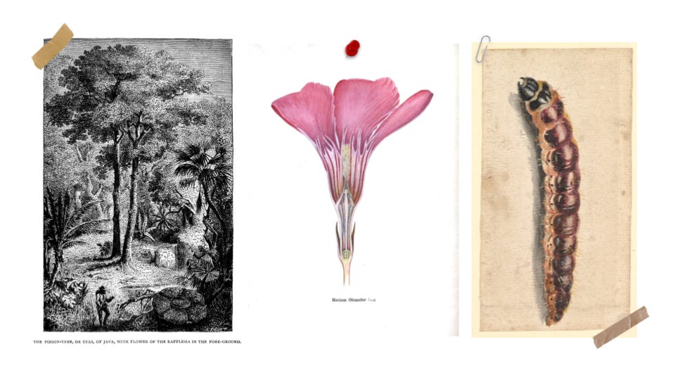 By Author — Not random images either, there’s a chance you find the compounds in all of these organisms.
Table of Contents #
- Exploratory Data Analysis for COCONUT — Profiling ~100K natural products to understand drug-likeness, physicochemical space, and screening viability.
- Chemical Similarity Search — Fingerprint-based filtering (ECFP, MACCS, pharmacophore, USRCAT) to reduce the database to high-similarity candidates.
- Protein Model Selection, Cleanup, and Preprocessing — Selecting acarbose-bound crystal structures and preparing them for docking.
- Protein–Ligand Docking & Assessment — Running GNINA-based virtual screening and scoring with CNN-VS.
- Lead Validation and Controls — Decoys, redocking replicates, statistical filtering, and stability analysis to remove false positives.
- Candidate Overview & Key Takeaways — Final shortlist by target protein and reflections on the workflow.
Flavonoids are a large, diverse group of secondary plant metabolites that play a role in pigmentation, UV protection, and insecticidal activity. Specifically, some anthocyanins (a subclass) can inhibit insect digestive enzymes, preventing nutrient uptake and development, serving as a defence mechanism against predators.
Obviously, there’s potential here for bug Ozempic (or insecticides, you pick). But research on Allium mongolicum flowers has also revealed that their flavonoids may inhibit human digestive enzymes, including our very own starch-metabolizing α-glucosidase. These compounds could be used to treat diabetes, as inhibiting starch breakdown reduces postprandial blood glucose levels (Li et al., 2025).
Initial docking analysis revealed that A. mongolicum-derived isoquercetin (already in clinical trials) can inhibit α-glucosidase (AGI) activity with an effect similar to that of acarbose , a common AGI derived from Actinoplanes bacteria. Chemical similarity search revealed that troxerutin (aka vitamin P4, a flavonoid you can buy over the counter) shares some substructural motifs with isoquercetin, and its docking analysis showed similar binding affinity.
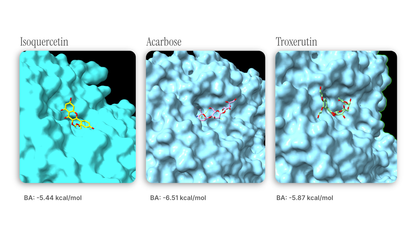 Docking results from DiffDock-Pocket.
Note : troxerutin’s slightly higher affinity may be attributed to steric interactions introduced by the moieties found on the larger molecule.
I wanted to take this approach and extend it to a larger database of natural compounds to find other biochemicals that could hypothetically outperform acarbose — after all, the drug is projected to have a $220 million global market by 2035.
Here’s my overall process:
Exploratory data analysis of COCONUT, a natural products database.
Chemical similarity search of acarbose against COCONUT to find structurally similar NPs.
Protein model selection, cleanup, and preprocessing.
Protein-ligand docking and assessment , where I run a virtual screen against human α-glucosidases.
Lead validation and controls to identify any false positives.
You can see all the code (in progress) here.
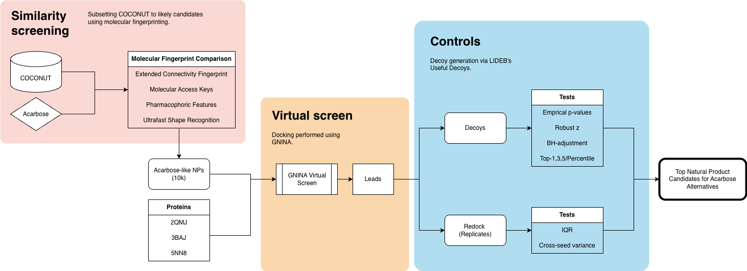 Workflow diagram
1. Exploratory data analysis for COCONUT #
In this section, I’ll take a look at:
Distributions of some pre-existing features in the database.
The spread of some derived ratios.
There are a little over 100,000 natural products in the COCONUT database. I started by doing some simple feature visualization:
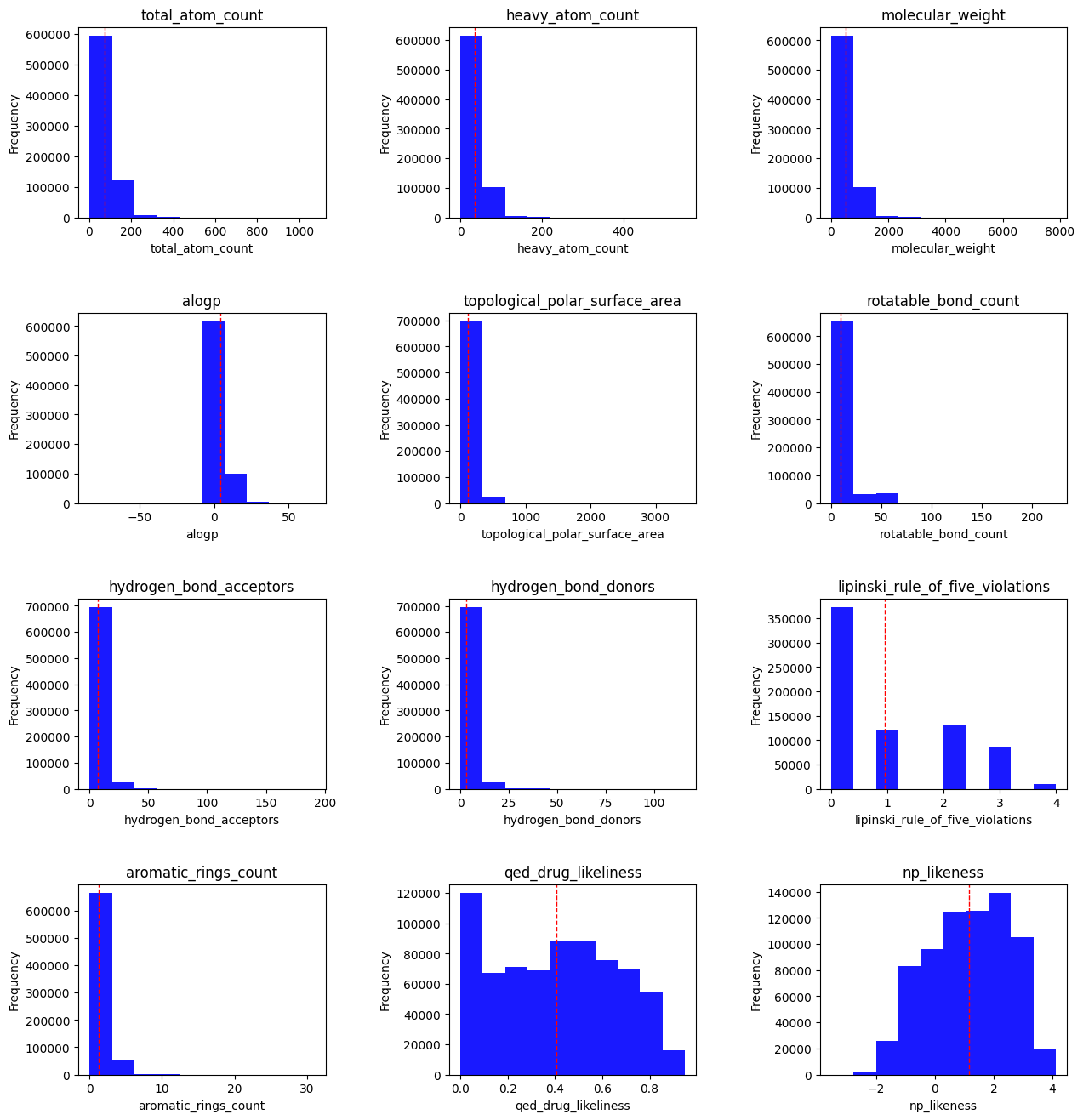
Total atom count : all atoms, including hydrogen.
Heavy atom count : any non-hydrogen atom.
Molecular weight : in grams per mole
ALogP : A drug discovery metric that estimates molecular lipophilicity.
Topological polar surface area : The surface sum of all polar atoms, also a measure for drug bioavailability.
Rotatable bond count : single bonds that allow for free rotation, generally a measure of flexibility/rigidity.
HBAs/HBDs : Polarity metrics — we typically want a particular balance of the two, with more HBAs than HBDs in drug-like molecules.
- Lipinski Rule of Five violations : the RO5 is a rule of thumb for evaluating drug-likeness based on a set of molecular properties. However, it is worth noting that several drugs do not have these characteristics — in other words, it is not the be-all and end-all. Those properties are:
- 5 or fewer HBDs
- No more than 10 HBAs
- Molecular mass under 500 Da
- ClogP < 5
Aromatic rings count : Aromatic rings add planarity to a molecule.
QED druglikeness : A drug likeness measurement that focuses on 8 features (all listed attributes other than RO5 and atom counts).
- NP likeness : Natural product likeness, measures a molecule’s similarity to known natural products.
For a closer look at some derived ratios, I looked at the following:
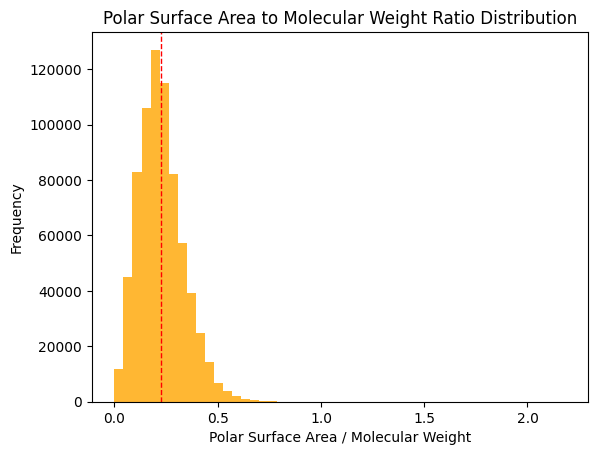
Research indicates that a TPSA/MW ratio >= 0.2 is ideal for good solubility; approximately half of the dataset meets this criterion (Whitty et al., 2018).
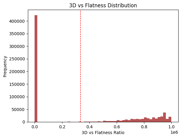
This metric stems from two findings:
Fsp3 (the fraction of sp3 carbons over total carbons) increases as drugs move through the discovery pipeline (Lovering et al., 2009).
Molecules with more than 3 rings tend to have poor solubility, high lipophilicity, and high promiscuity (i.e., off-target binding) (Ritchie et al., 2011).
Here, I take the ratio of both in the dataset. Two populations emerge: many NPs with no saturated carbons and a smaller group with some balance.
Takeaways :
- COCONUT offers a relatively diverse search space
- There appears to be drug-like potential amongst several NPs
2. Chemical similarity search #
Chemical similarity is generally determined by generating chemical fingerprints for a molecule, fixed-size identifiers that capture information about atomic structure and chemistry. Several fingerprinting protocols exist, each with its own strengths and weaknesses. Here are the ones I chose and why:
ECFP. Extended-Connectivity Fingerprints represent molecular structures and are widely used in cheminformatics. They enable substructure and similarity searching but are also used for quantitative structure-activity relationship (QSAR) modelling. If you’re interested in molecular activity, these are a good pick.
Pharmacophoric features. These fingerprints encode data on chemical features typically involved in pharmacological actions, such as hydrophobicity, charge, aromaticity, etc. This makes them useful when we’re looking for chemicals with properties similar to those of acarbose.
MACCS keys. Short for Molecular Access System, MACCS are one of the simpler fingerprinting methods. They encode the answers to established T/F questions about chemical structures, such as the ring size, ion presence, or oxygen count. They can be generated quite quickly and are relatively interpretable.
Ultrafast Shape Recognition. USR is the only 3D method on this list. It generates a vector of shape descriptors for a set of conformers of a given molecule. USRCAT, which I am using more specifically, also encodes pharmacological features.
By generating fingerprints for acarbose, we can use Tanimoto similarity to assess the degree of agreement between our database compounds and the lead target. USR is the exception; we use inverse Manhattan distance instead.
To trim the dataset down, I used the following cutoffs for Tanimoto similarity:
ECFP: 0.4. Research seems to show enrichments of similarly active compounds beyond a TC of 0.4 with minimal false positives.
MACCS: 0.7. See above.
Pharmacophoric features: 0.8. A slightly more arbitrary cutoff, but I elected to be stricter since ECFP and MACCS are fairly generous.
USRCAT: top 1%. In virtual screening workflows and decoy comparison benchmarks, the top 1% of candidates are selected.
This gave me a dataset of 10,341 high-similarity candidate molecules to explore. Ligands were generated using RDKit and converted to .pdbqt using OpenBabel.
3. Protein model selection, cleanup, and preprocessing #
Acarbose is a bit of a rolling stone, it can’t be tied down — by which I mean it interacts with multiple proteins. To be thorough, I wanted to explore this virtual screening process across all of its protein targets at once. In hindsight, this made it much harder to keep track of (I’ll take it one target at a time from now on).
I made my selections based on protein targets listed in DrugBank and the resolution of the corresponding protein model. I also specifically selected PDB entries of the target protein _ in complex with acarbose_ so I’d a) have a defined binding pocket and b) have an experimental reference point for future validations. Finally, all proteins were put through PDB-redo before being converted to .pdbqt for docking:
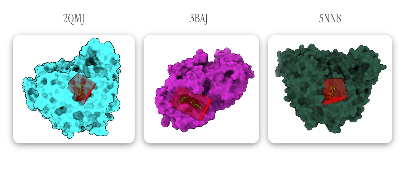
- 2QMJ : The N-terminal subunit of human maltase-glucoamylase in complex with acarbose. As you can see from the PDB page, there’s room for growth in model quality, but PDB-redo led to some minor improvements. (Gene: MGAM).
- 3BAJ : Human pancreatic alpha-amylase in complex with nitrate and acarbose. PDB-redo led to more significant improvements here. (Gene: AMY2A).
- 5NN8 : Human lysosomal acid-alpha-glucosidase in complex with acarbose (Gene: GAA).
Below, acarbose is designated in light green with binding residues (within 4 Å of acarbose) in red. All other observed elements are ions and ligands, which are removed for docking.
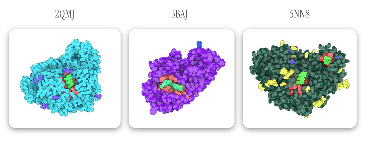 Note: one of the highlighted light green ligands in 5NN8 is an acarbose-derived trisaccharide; the other binding pocket (containing true alpha-acarbose) is used for docking configuration — Images generated via The Protein Imager.
4. Protein-ligand docking & assessment #
 Figures generated using ChimeraX. Can you tell I tried (unsuccessfully) to create Goodsell-like graphics?
For protein-ligand docking, I usedGNINA, an open-source AutoDock Vina fork that uses CNNs to score ligand poses.
Since we know where acarbose is supposed to bind (the protein models include acarbose), we can guide the docking process by setting an autobox (basically a mini 3D search space) around its coordinates. In the diagrams above, I’ve indicated the autobox GNINA draws around the ligands (4 Å outward from the farthest corners of the molecule) in red.
While it may be the most computationally expensive step, this stage of the project was actually the easiest. I ran GNINA on an HPC cluster in parallel fashion to save time — although GNINA wasn’t designed specifically for high-throughput virtual screening1, this step was completed in approximately one day.
5. Lead validation and controls #
In this section, I go over:
Filtering through the results of our initial docking run.
Analyzing the results of decoy docking tests.
Compare lead ligand performance across replicates.
GNINA generates several metrics for binding poses , including CNN pose score (the AI’s assessment for score quality) and CNN binding affinity (the AI-predicted kcal/mol). Benchmarking studies with GNINA have indicated that the product of these two values, CNN_VS (virtual screening), can be used to identify potentially active ligands when it exceeds 6.30.
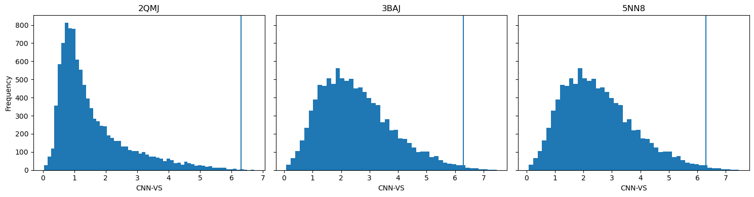 Horizontal lines represent the CNN-VS threshold of 6.30.
Taking the CNN_VS of all ligands docked against each protein, 71 ligands passed the threshold.
Okay, the headline promise-payoff is complete—but we’re not done yet. After collecting a set of leads, I needed to validate some of the findings. There were a few ways I went about doing this, with each control telling me something different:
Molecular decoys. For each lead, I used LUDe to generate physicochemically similar molecules for docking against the protein receptors. Decoy molecules tell us whether there’s something unique about a lead or if any molecule with a similar molecular weight, log P, polarity, etc., would perform just as well.
Redocking with variant seeds. By using different seeds, we can check whether the results from our first run are consistent or a fluke — in other words, we need to run replicates.
Structural interaction fingerprint comparison. The PLECFP, or protein-ligand extended connectivity fingerprint, is a method for hashing protein-ligand interactions for comparison. Here, I used it to compare structural interactions between the leads and acarbose during protein binding.
Here are the results for each:
Molecular decoys #
Decoys help us determine whether our docking results are false positives. By matching our lead molecules against decoy molecules with similar properties (e.g., molecular weight, number of rotatable bonds, log P), we can assess whether our leads have real potential.
I used LUDe (LIDEB’s Useful Decoys) to generate decoys for all (putatively) biologically active ligands. LUDe provides fifty decoys per ligand, all of which were docked against the protein models using GNINA under the same parameters, with CNN-VS taken as well.
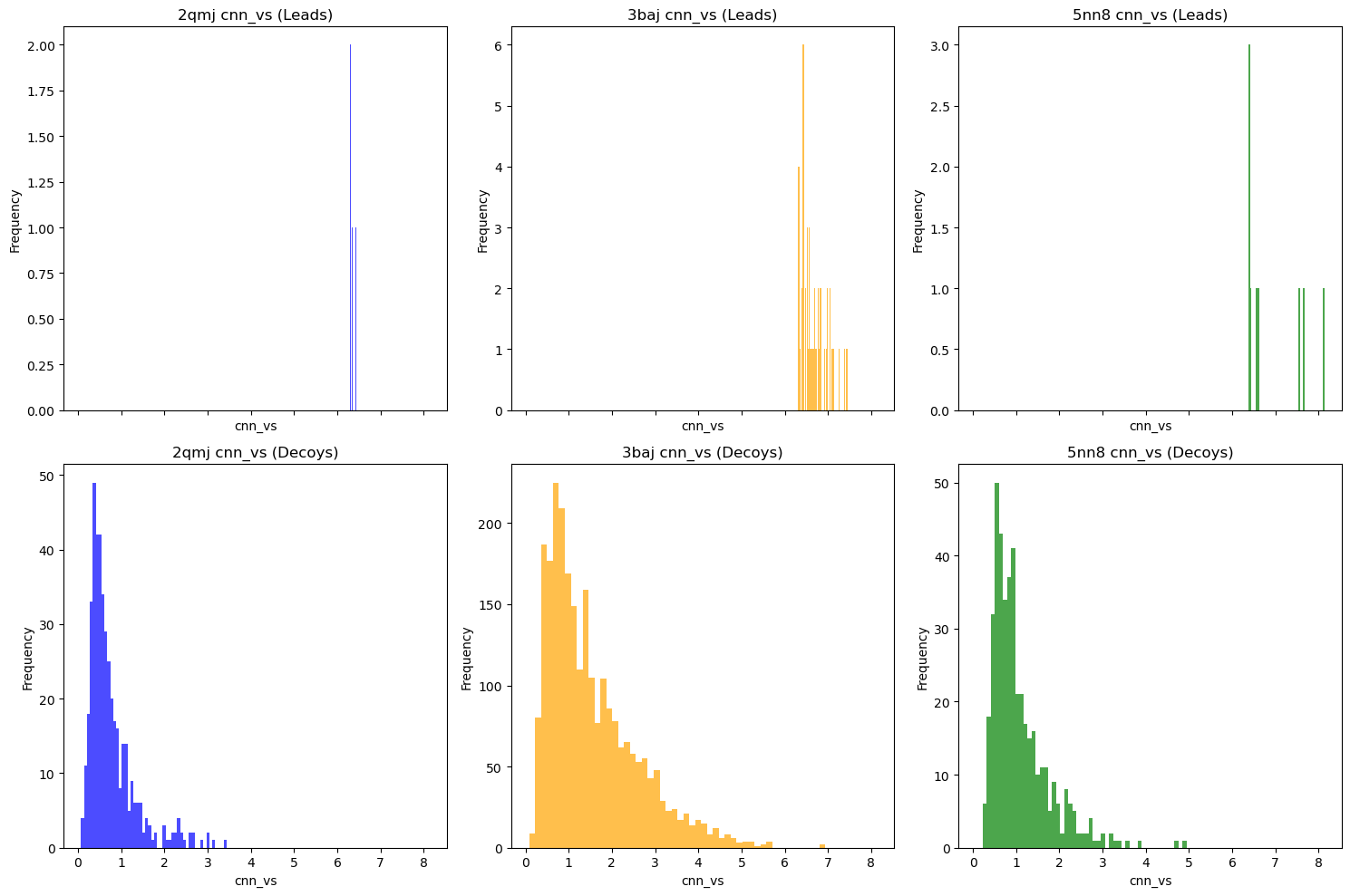 Comparative overall performance (measured via CNN-VS) of leads vs. property-matched decoys.
Alternatively:
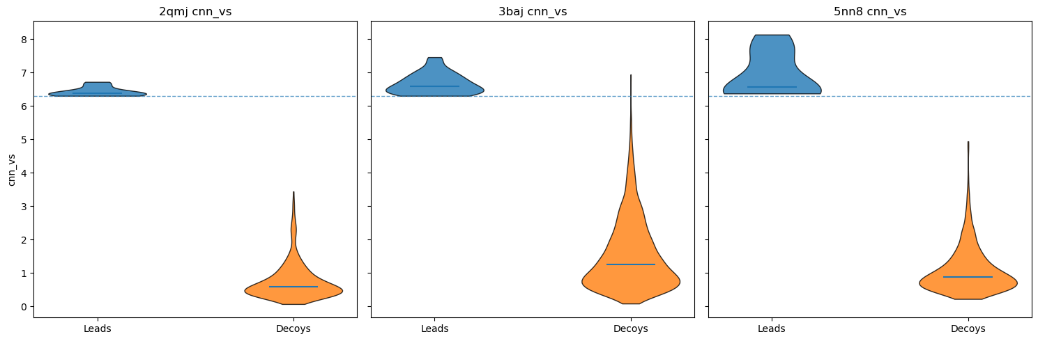
As you can see, nearly all decoy poses scored below our activity threshold. However, to be more robust, I did the following checks:
Get a one-sided empirical p-value, robust z-score, and Benjamini-Hochberg adjusted q-value for each ligand vs. decoy set.
Determine the top-1 enrichment for each ligand vs. decoy set (or, how often does the ligand outrank its decoys in CNN-VS).
P-values & z-scores #
For each ligand, I compared CNN-VS scores with ~50 matched decoys (in some cases, RDKit was unable to generate conformers for the decoys) and computed a one-sided empirical p-value. I also determined how many robust standard deviations the ligand lay above the median and adjusted all p-values using the Benjamini-Hochberg false discovery rate.
2QMJ & 5NN8: For all ligands, all adjusted p-values < 0.05.
3BAJ : Out of 53 ligands, one p-value > 0.05.
Some results for 3BAJ are shown below.
Ligand dominance, or rank-based enrichment #
Realistically, the ligand vs. decoy sets are too small for any real statistical robustness. A more useful heuristic is to compare the ligands’ ranks relative to their matched decoys when ordered by CNN-VS.
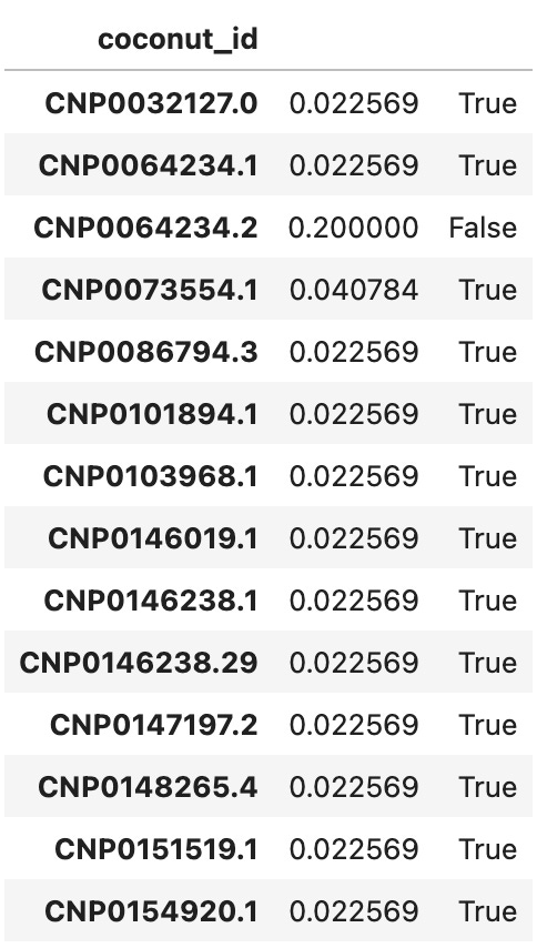
For all three proteins, all leads ranked at or above the 98th percentile relative to their decoys. Actually, all except 2 leads for 3BAJ ranked first relative to their decoys. Some results for 3BAJ are shown below:
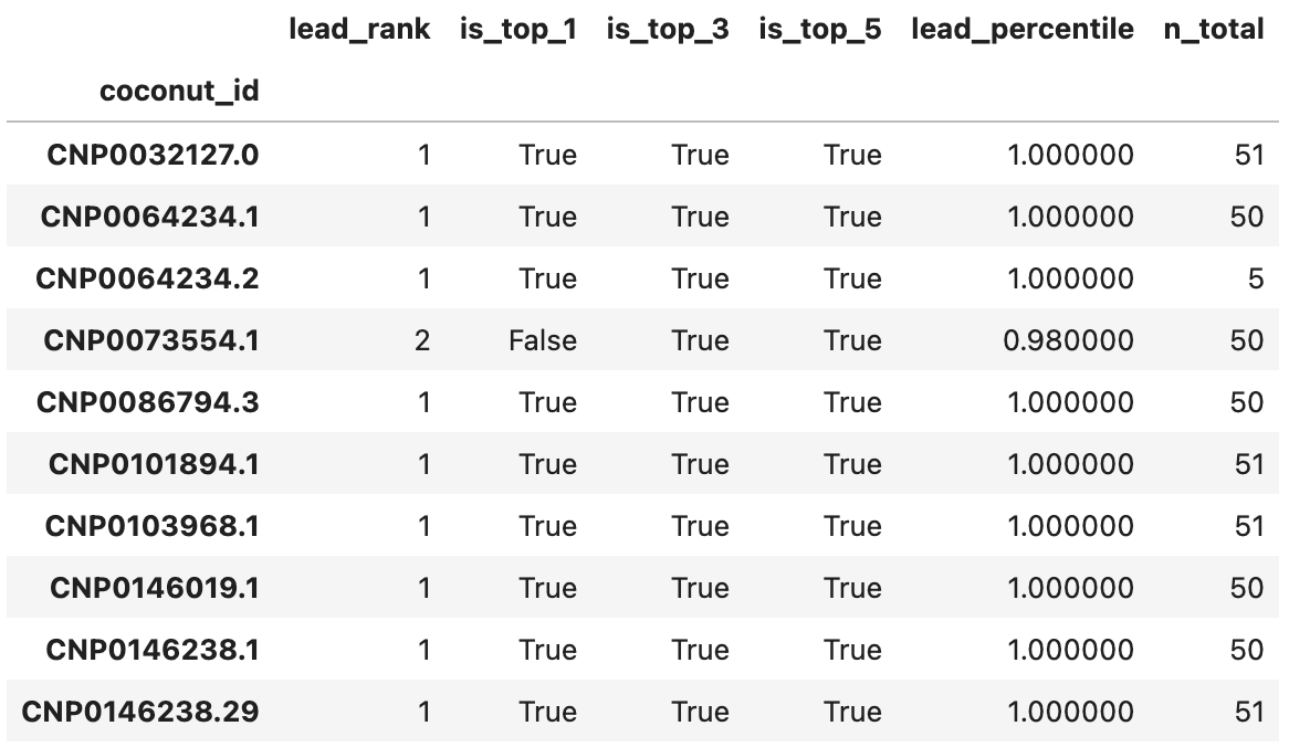 You’ll notice very few decoys were generated for CNP0064234.2; it was not considered a candidate for 3BAJ.
Redocking with variant seeds #
One of the more important validation tests, this process is meant to tell us if the leads we determined were flukes or are consistently high-CNN-VS across replicates , an attribute we’ll refer to as stability from here on.
Once again, this control helps us filter out false positives. If expanded, it can help us identify false negatives: ligands that didn’t pass the CNN-VS threshold in the original screen but would otherwise. I chose not to do that in this project due to time and computational cost constraints, but it would be a logical next step.
For this control, I simply took all of our leads and docked them again with GNINA using 5 variant seeds. Below are the distributions of CNN-VS scores for the initial run compared with the redocked runs:
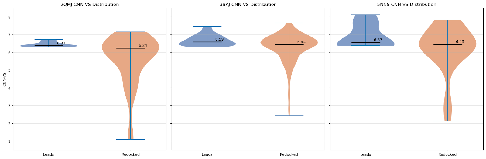
As we can see, the CNN-VS for the redocked ligands exhibits a wider distribution (as expected — we haven’t artificially subset them to CNN-VS >= 6.30, and there are 25 times as many data points).
Let’s take a closer look:
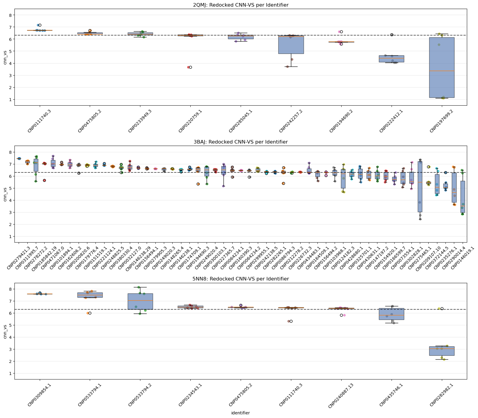 5.1. Jittered Box-Plot of CNN-VS Distribution by Identifier Across All Seeds
What this shows:
Each box shows the spread of CNN-VS scores for a given lead identifier across all seeds, including the original and redocking runs.
Identifiers are ranked by median CNN-VS.
This gives us a sense of consistency vs variance per ligand.
Already, we can see several leads do not pass muster.
Why it matters:
These charts help us see which identifiers have the most consistent CNN-VS scores and whether their distributions exceed the biologically active threshold.
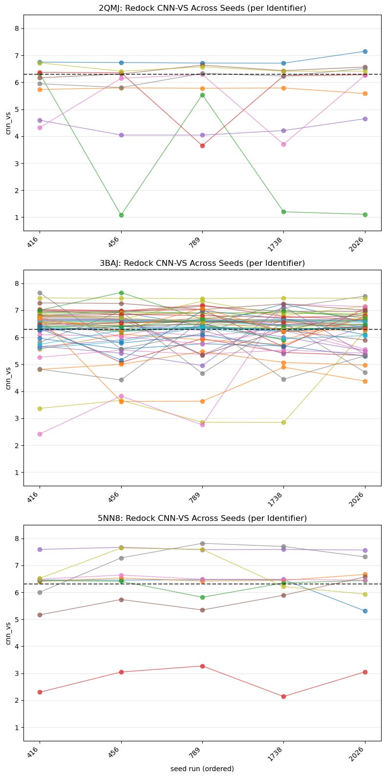 5.2. Spaghetti Plot of Best CNN-VS Score by Identifier Across All Seeds
What this shows :
This is a closer look than the previous boxplot and shows us seeds on the x-axis. Once again, it shows us the consistency and potency of each identifier:
Which ligands are seed-stable vs. seed-sensitive?
How often are trajectories exceeding 6.30?
Are high medians due to lucky seeds or consistency?
Note : It might make more sense to use a spaghetti plot for fewer samples that were actually labelled, but here it’s meant to provide a broader overview.
Why it matters :
These plots show whether CNN-VS scores are consistent across runs and how high or low those scores are. We’re looking for consistent scoring that’s also above the threshold.
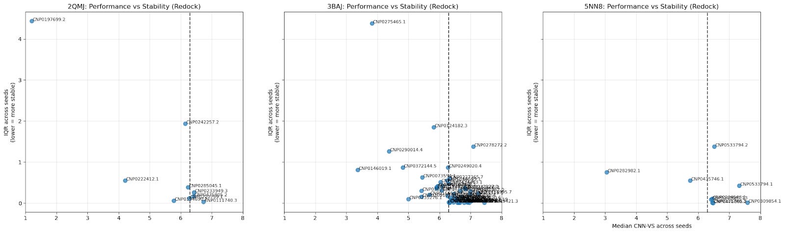 5.3. Scatter Plot of Cross-Seed Median CNN-VS Score & Cross-Seed Interquartile Range
What this shows :
The median CNN-VS across seeds provides a general idea of the CNN-VS for a particular ligand; the IQR indicates the stability of that CNN-VS. A lower IQR means a tighter distribution.
Bottom-right quadrant: low variance, high CNN-VS (most promising candidates).
Top-right quadrant: high variance, high CNN-VS (false positives).
Top-left quadrant: high variance, low CNN-VS (discard).
Bottom-left quadrant: low variance, low CNN-VS (true negatives)
Are high medians due to lucky seeds or consistency?
Why it matters :
This is another way of visualizing consistency (low IQR) and quality (median CNN-VS).
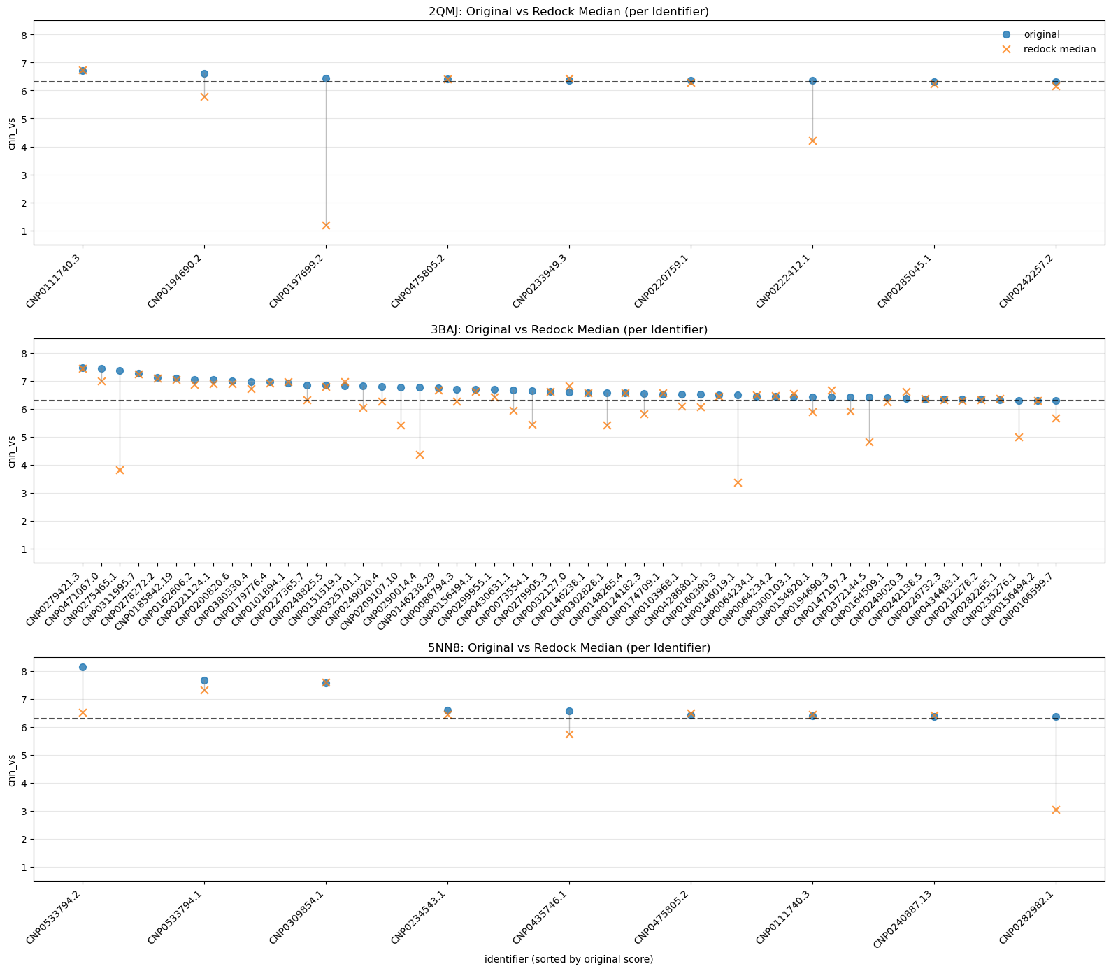 5.4. Median Comparison Between Originals and Redock CNN-VS by Identifier
What this shows :
One of the simpler visualizations; all we see here is the difference between the original run’s CNN-VS and the median redock runs’ CNN-VS.
A small drop tells us our original run for that ligand was reliable.
A big drop means it got lucky.
This plot becomes more useful if we expand our initial redocking set to include those leads with CNN-VS scores below 6.30 — a jump would indicate a false negative.
Why it matters :
A companion to IQR vs. CNN-VS. A snapshot of pose stability.
Taking all of this into account, my final filtration process was to subset to the leads that scored CNN-VS > 6.30 in 5 out of 6 replicates, then rank them by the median CNN-VS-to-interquartile range ratio. That meant the top 3 candidates for each protein were as follows:
2QMJ :
CNP0111740.3
CNP0475805.2 (Phaeospelide A)
CNP0233949.3 (Convallataxol)
3BAJ :
CNP0242138.5
CNP0146238.1
CNP0185842.19
5NN8 :
CNP0533794.1
CNP0234543.1 (2-deoxyecdysterone 20,20-monoacetonide)
CNP0111740.3
We’ll take a closer look at these soon — but first, let’s do one final validation.
Structural interaction fingerprint comparison #
The goal of this step is more exploratory than confirmatory. My aim here was to determine whether the lead ligands interact with the target proteins similarly to experimental acarbose. We don’t exactly need to prioritize the ligands with similar binding profiles, as it could be expected that a more performant ligand would behave differently.
We can compare ligand-protein structural interactions across a diverse set of ligand sizes using structural interaction fingerprints. These go one step beyond typical molecular fingerprints and encode molecular interactions between ligands and binding-pocket residues, hashing them to preset sizes to enable comparisons.
It seems the best fingerprint so far isPLECFP, which combines the best features of all previous methods — atomic environment capture, expanded capture radius, etc. It’s shown promise in AI tasks, lead optimization, and scaffold hopping. That’s why I chose to use it for my initial pass:
As you can see, our similarity scores are practically zero. (Full disclosure: this was a pretty disappointing chart to generate).
These results are a little surprising — the initial list of 10,000 candidates was selected because they shared similarities with acarbose, so we’d expect at least some overlap.
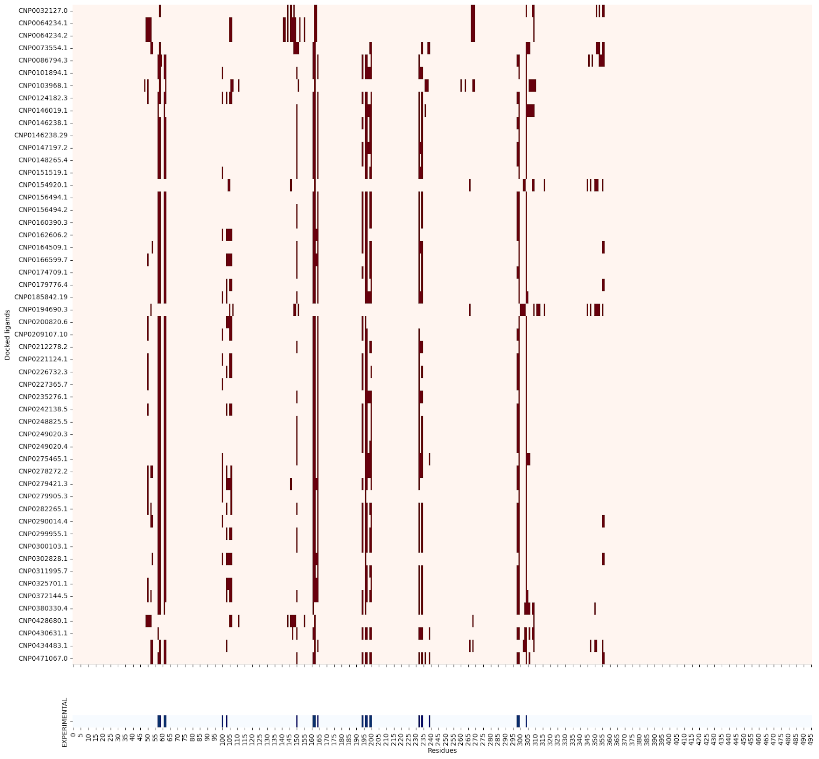
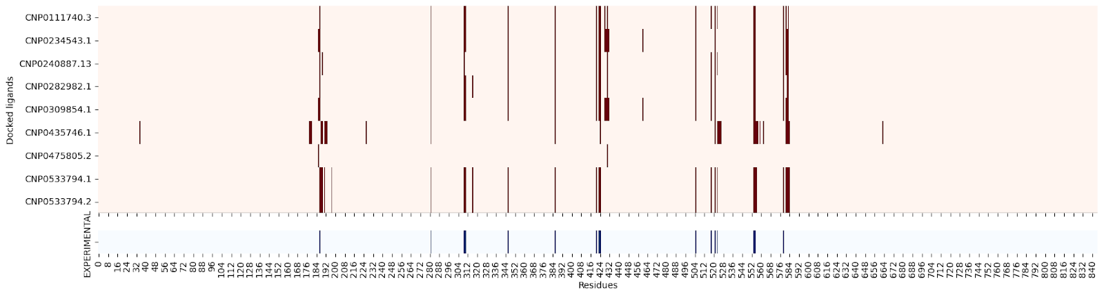
Moreover, when creating a residue contact map for each ligand against its target protein, the interacting residues seem quite similar:
2QMJ :
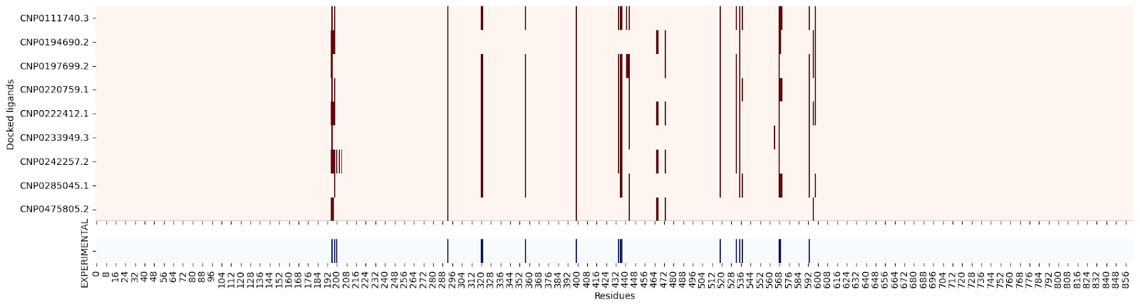
3BAJ :
5NN8 :
I’m still not sure why this might be, so please let me know if you have an explanation!
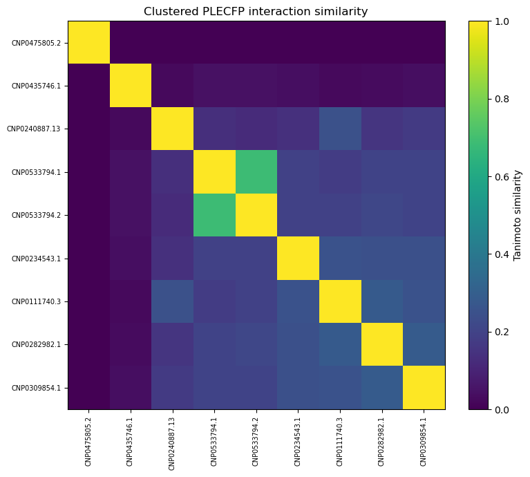
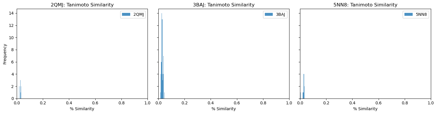
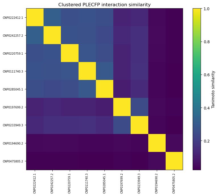
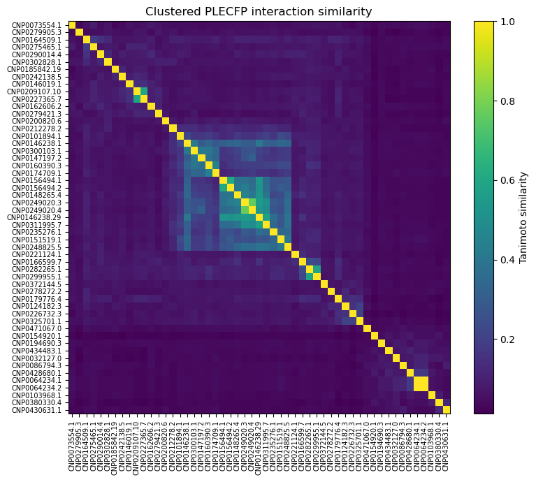
Also, out of curiosity, I determined pairwise Tanimoto similarity across all leads2. There seems to be clustering among some 3BAJ leads, which may merit further investigation.
Some of the lead ligands for 3BAJ, such as CNP0146238.29, appear to share binding behaviours with other leads, such as CNP0156494 — this may be something worth further investigation.
Candidate overview & key takeaways #
Let’s start by interpreting our shortlist from earlier:
2QMJ #
CNP0111740.3 : An oleanane triterpenoid that shares parentage with Ilekudinoside I, and seems to appear in traditional Chinese medicine.
CNP0475805.2 (Phaeospelide A): A polyene macrolide from Arthrinium phaeospermum , a hairy-caterpillar-associated fungus. Although the genes required to express this molecule appear silent in the fungus, they were heterologously expressed in bacteria. This molecule also exhibits binding affinity with 5NN8.
CNP0233949.3 (Convallataxol): The best-annotated NP on this list, convallataxol, is a steroid glycoside found in the leaves and flowers of Antiaris toxicaria , a highly poisonous tree.
3BAJ #
CNP0242138.5 : Another cardenolide from the Nerium indicum and Nerium oleander species, flowering shrubs used in traditional medicine.
CNP0146238.1 : An ecdysteroid that appears to be used in Ethiopian traditional medicine.
CNP0185842.19 : A cardenolide that seems to be a stereo variant of beauwalloside, which is also found in N. oleander.
5NN8 #
CNP0533794.1: An open-chain polyketide — no other documentation found.
CNP0234543.1 (2-deoxyecdysterone 20,20-monoacetonide): An ecdysteroid from the roots of the Silene brahuica plant, shown to have some anti-inflammatory properties.
CNP0111740.3 (See earlier)
Some honourable mentions:
CNP0156494.1 : An ecdysteroid from Vitex polygama , which appears to be shidasterone, which seems to have enzyme-inhibitory effects.
CNP0279421.3 : Torvoside K, a saponin from many species, including ones of the Solanum genus, which seems to have antifungal properties.
If you’re in a lab, made it this far, and have access to such delightful flora as A. toxicaria or a library of traditional Ethiopian medicine, feel free to take this list of lead candidates and get to testing.
Some of my key takeaways:
The easiest part of virtual screening is the docking. The real work involves preparation, preprocessing, post-docking controls, and validation.
Many natural products lack sufficient research, even though they present countless therapeutic opportunities. Admittedly, this is largely due to extraction and isolation challenges — but there’s an opportunity here nonetheless.
Good research involves lots of small, smart decisions. Several times during this project (not documented here), I had to back up and redo an entire step after rushing through a small decision. Better planning and research ahead of time would have saved time and boosted my efficiency.
Thank you for reading! Am I a genius? A modern Prometheus? Have I made grievous and unforgivable scientific errors? Please let me know if you have any feedback.
They actually specifically recommend against using GNINA for high-throughput screening applications. However, simple parallelization allows you to spawn multiple GNINA processes on a single GPU node, so you can take advantage of the program’s speed.
2BAJ :
3BAJ :
5NN8: